4What is optimization?

In this chapter we will denote the set of column vectors with $d$ rows by $\mathbb{R}^d$ . The arithmetic of $d\times 1$ matrices apply i.e., we may add vectors in $\mathbb{R}^d$ and multiply them by a number in $\mathbb{R}$ .

In the next chapter we will introduce them as euclidean vector spaces. The term euclidean refers to a norm: a function measuring the size of a vector. In this chapter we only need the structure as column vectors.

4.1 What is an optimization problem?

An optimization problem consists of maximizing or minimizing a function subject to constraints.

Below are two classical examples related to minimizing (non-linear) functions subject to (non-linear) constraints. These are actually examples of convex optimization problems. More about that later.

A cylindrical can is supposed to have a volume of $V$ $\text{m}^3$ . The material used for the top and bottom costs $T$ DKK per $\text{m}^2$ and the material used for the side costs $S$ DKK per $\text{m}^2$ . Give the dimensions $r$ and $h$ of the can minimizing the price of the materials.

The cost of the top and bottom pieces are $2 \pi r^2 T$ . The cost of the side material is $2\pi r h S$ . The constraint is that the volume must be $V$ . This is expressed in the equation $\pi r^2 h = V$ . All in all the optimization problem is

$\begin{aligned} &\text{Minimize} &2\pi r^2 T + 2\pi r h S&\\ &\text{with constraints}\\ &&\pi r^2 h &= V\\ &&r &\geq 0\\ &&h &\geq 0, \end{aligned}$ where $V, T$ and $S$ are constants.

Can you see a way of solving this optimization problem by eliminating $h$ in the constraint $\pi r^2 h = V$ ?

Hint

$\pi r^2 h = V\iff h = \frac{V}{\pi r^2}$ and $h$ can be inserted in $2\pi r^2 T + 2 \pi r h S$ . Why is this helpful?

A person is in distress $D$ meters from the beach. The life guard spots the situation, but is $d$ meters from where he would naturally jump in the water as indicated below. The life guard runs $8$ m/s on the beach and swims $1$ m/s in the water. How far ( $x$ ) should he run along the beach before jumping into the water in order to minimize the time needed to reach the person in distress?

The time spent moving with a speed of $v$ over a distance of $s$ is

$t = \frac{s}{v}.$ If the life guard jumps in the water at the point $x$ he will have to swim a distance of

$\sqrt{D^2 + (d-x)^2}$ using the Pythagorean theorem. Therefore the optimization problem becomes

$\begin{aligned} &\text{Minimize} &\frac{x}{8} + \sqrt{D^2 + (d-x)^2}&\\ &\text{with constraints}\\ &&x\geq 0\\ \end{aligned}$ Strictly speaking we do not need the constraint $x\geq 0$ , as the life guard is free to run in the other direction. So the optimization problem is simply to minimize

$\frac{x}{8} + \sqrt{D^2 + (d-x)^2}$ with no strings attached i.e., $x\in \mathbb{R}$ is just assumed to be any number.

You need to build a rectangular fence in front of your house for a herb garden. Your house will make up one side of the rectangle, so you only need to build three sides. Suppose you have 10 m of wire. What is the maximum area of the herb garden you can wall in?

4.2 General definition

An optimization problem consists of a subset $D\subseteq \mathbb{R}^d$ and a function $f:D\rightarrow \mathbb{R}$ . We will consider optimization problems in the context of minimization. Optimize in this situation means minimize.

In our most general setting an optimization problem looks like

$\begin{aligned} &\text{Minimize} &f(x)&\\ &\text{with constraint}\\ &&x\in C, \end{aligned}$ where $C$ and $D$ are subsets of $\mathbb{R}^d$ with $C\subseteq D$ and $f: D\rightarrow \mathbb{R}$ is a function. A solution to the optimization problem is a vector $x_0\in C$ , such that

$f(x_0) \leq f(x)$ for every $x\in C$ . Here $x_0$ is called an optimum and $f(x_0)$ is called the optimal value.

We will often write the optimization problem defined above in short form as

$\begin{aligned} &\text{min}\, f(x)\\ &x\in C. \end{aligned}$

The complexity of the problem depends very much on the nature of $C$ and $f$ . Also, we cannot even be certain that an optimization problem has a solution. Consider the problem

$\begin{aligned} &\text{min}\,x\\ &x\leq 0 \end{aligned}$

Here $x$ can be made arbitrarily small subject to the constraint $x\leq 0$ and the problem has no solution.

We have deliberately not included maximization problems in Definition 4.5. This is because a maximization problem, such as

$\begin{aligned} &\text{Maximize} &f(x)&\\ &\text{with constraint}\\ &&x\in C \end{aligned}\tag{4.1}$

can be formulated as the minimization problem

$\begin{aligned} &\text{Minimize} &-f(x)&\\ &\text{with constraint}\\ &&x\in C. \end{aligned}\tag{4.2}$

Again, we will use the short notation

$\begin{aligned} &\text{max}\,f(x)\\ &x\in C \end{aligned}$ for the maximization problem in (4.1). A solution to (4.1) is a vector $x_0\in C$ , such that

$f(x_0) \geq f(x)$ for every $x\in C$ . Again, $x_0$ is called an optimum and $f(x_0)$ the optimal value.

Suppose that the maximization problem

$\begin{aligned} &\text{max}\, f(x)\\ &x\in C \end{aligned}\tag{4.3}$ is formulated as the minimization problem

$\begin{aligned} &\text{min}\, -f(x)\\ &x\in C. \end{aligned}\tag{4.4}$ Show that $f(x_0)$ is the optimal value and $x_0$ the optimum for (4.3) if $-f(x_0)$ is the optimal value and $x_0$ the optimum for (4.4).

Suppose that $a > 0$ . Solve the optimization problem

$\begin{aligned} &\text{Minimize} &a x^2 + b x + c\\ &\text{with constraint}\\ &&x\in \mathbb{R}. \end{aligned}$

4.3 Convex optimization

Particularly well behaved optimization problems are the convex ones. These are optimization problems, where $C\subseteq \mathbb{R}^d$ is a convex subset and $f:C\rightarrow \mathbb{R}$ a convex function in Definition 4.5. To define these concepts we first introduce the notion of a line in $\mathbb{R}^d$ .

A line $L\subseteq \mathbb{R}^d$ is a subset of the form

$L = \{u + t v \mid t\in \mathbb{R}\},$ where $u, v\in \mathbb{R}^d$ with $v\neq 0$ .

A line $L$ in the plane $\mathbb{R}^2$ is (usually) given by its equation

$y = a x + b. \tag{4.5}$ This means that it consists of points $(x, y)\in \mathbb{R}^2$ satisfying $y = a x + b$ . Here $a$ can be interpreted as the slope of the line and $b$ the intersection with the $y$ -axis.

What about all the points $(x, y)$ with $x = 0$ ? Certainly they also deserve to be called a line. However, they do not satisfy an equation like (4.5). Informally, this line has infinite slope.

Therefore we introduce the parametric representation of a line: a line is the set of points of the form

$\begin{pmatrix} x_0 \\ y_0 \end{pmatrix} + t \begin{pmatrix} u_0 \\ v_0 \end{pmatrix}, \tag{4.6}$ where $t\in \mathbb{R}$ ,

$\begin{pmatrix} x_0 \\ y_0\end{pmatrix}$ is any point on the line and

$\begin{pmatrix} u_0 \\ v_0\end{pmatrix}$ is a non-zero (directional) vector.

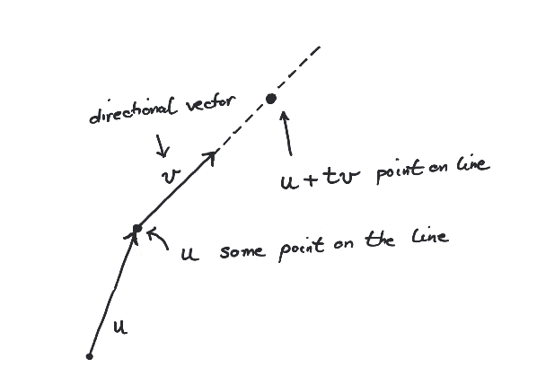
Example of a line in $\mathbb{R}^2$ with (directional) vector $v\in \mathbb{R}^2$ through the point $u\in \mathbb{R}^2$ .

Given two distinct points

$\begin{pmatrix} x_0 \\ y_0 \end{pmatrix} \qquad\text{and}\qquad \begin{pmatrix} x_1 \\ y_1 \end{pmatrix},$ there is one and only one line passing through them. This line is given by

$\begin{pmatrix} x_0 \\ y_0 \end{pmatrix} + t \begin{pmatrix} x_1 -x_0\\ y_1-y_0 \end{pmatrix}. \tag{4.7}$

How do we convert the line $y = a x + b$ in (4.5) to the parametric form (4.6)? Well, we know that the two distinct points

$\begin{pmatrix} 0 \\ b \end{pmatrix}\qquad\text{and}\qquad \begin{pmatrix} 1 \\ a + b \end{pmatrix}$ are on the line. Therefore it is given by

$\begin{pmatrix} 0 \\ b \end{pmatrix} + t \begin{pmatrix} 1 \\ a \end{pmatrix}$ by (4.7).

Mentimeter

Line directional vector

Compute the parametric representation of the line $L$ through the points $(1, 1)$ and $(2, 3)$ . Also compute $a$ and $b$ in the representation $y = a x + b$ for $L$ .

What is the parametric representation of the line consisting of the points $(x, y)$ with $x=0$ ?

Show in Definition 4.9 that if $L$ is given by $u$ and $v$ , then you might as well replace $v$ by $s v$ , where $s$ is a real number and $s\neq 0$ . It gives the same line.

Show that there is a unique line passing through two distinct points $x, y\in \mathbb{R}^d$ and that it is given by $u = x$ and $v = y - x$ in Definition 4.9.

Do the points

$\begin{pmatrix}1\\ 2\\ 3\end{pmatrix}, \quad \begin{pmatrix} 4\\ 5\\ 6\end{pmatrix} \quad\text{and}\quad \begin{pmatrix} 7\\ 8\\ 9\end{pmatrix}$ lie on the same line in $\mathbb{R}^3$ ?

Show that the line through two distinct points $x, y\in \mathbb{R}^d$ is equal to the subset

$\{ (1-t) x + t y \mid t\in \mathbb{R}\} \subseteq \mathbb{R}^d.$

A convex subset $C\subseteq \mathbb{R}^d$ is a subset that contains the line segment between any two of its points $x, y\in C$ i.e.,

$(1 - t) x + t y\in C$ for every number $t$ with $0\leq t \leq 1$ .

Example of non-convex subset of $\mathbb{R}^2$ .

Which of the subsets below are convex?

$C=\{1\}\subseteq \mathbb{R}$

$C=\{1, 2\}\subseteq \mathbb{R}$

The points $C$ on a line $y = a x + b$ in $\mathbb{R}^2$ .

$C=\{(x, y)\in \mathbb{R}^2 \mid x y \geq 0\}.$

A closed interval in $\mathbb{R}$ is a subset of the form

$[a, b] = \{x \mid a \leq x \leq b\}$ for $a \leq b$ . Prove that $[a, b]$ is a convex subset of $\mathbb{R}$ .

Hint

Keep cool and just apply the definitions! First of all, $x\in [a, b]$ if and only if

$a\leq x \land x \leq b. \tag{4.8}$ Now pick any $t\in [0, 1]$ . We must show that if $x\in [a, b]$ and $y\in [a, b]$ , then

$(1 - t)x + t y \in [a, b].$ You may also write this out as

$a\leq x \land x \leq b\qquad\land\qquad a\leq y \land y \leq b$ implies that

$a\leq (1 - t)x + t y \qquad \land \qquad (1 - t)x + t y \leq b.$

Hint

$a\leq x\implies (1-t) a \leq (1-t) x\qquad\land\qquad a\leq y \implies t a \leq t y$ implies that

$(1 - t) a + t a \leq (1-t)x + t y.$ What is $(1-t)a + t a$ ?

Let $A$ and $B$ be convex subsets of $\mathbb{R}^d$ . Prove that $A\cap B$ is a convex subset of $\mathbb{R}^d$ . Generalize this to show that if $A_1, \dots, A_n$ are any number of convex subsets of $\mathbb{R}^d$ , then their intersection

$A_1 \cap \cdots \cap A_n$ is a convex subset of $\mathbb{R}^d$ . Is the union of two convex subsets necessarily convex?

A convex function is a function $f: C\rightarrow \mathbb{R}$ defined on a convex subset $C\subseteq \mathbb{R}^d$ , such that

$f((1 - t) x + t y) \leq (1-t) f(x) + t f(y)$ for every number $t$ with $0\leq t \leq 1$ .

Graph of convex function. The line segment between $(x, f(x))$ and $(y, f(y))$ lies above the graph.

Let the function $f: \mathbb{R} \rightarrow \mathbb{R}$ be given by $f(x) = a x + b$ , where $a, b\in \mathbb{R}$ . Show that $f$ is a convex function.
Hint
Try the case $a = 0$ first.
Can you at this point prove that $f(x) = x^2$ is a convex function?
Hint
Simplify
$(1 - t) x^2 + t y^2 - ((1-t) x + t y)^2$ to an expression that has to be non-negative.
Hint
Using that $f(x) = x^2$ is a convex function, prove that $g(x) = x^4$ is a convex function.
Hint
Use that $g(x) = f(x)^2$ and $a \leq b\implies a^2 \leq b^2$ if $a, b\geq 0$ (here we really need $a, b\geq 0$ , since for example $-2 \leq -1$ , but $4 \leq 1$ is not true) to conclude that
$((1-t) x + t y)^4 = (((1-t)x + t y)^2)^2 \leq ((1-t)x^2 + t y^2))^2 \leq (1-t) x^4 + t y^4$ for $x, y\in \mathbb{R}$ .
It is a fact that $f(x) = x^3$ is not a convex function, but can you explain this using the definition of a convex function?
Hint
Try $x = -1, y = 0$ and $t =\frac{1}{2}$ .

Let $f: \mathbb{R}^d\rightarrow \mathbb{R}$ be a convex function. Then the subset

$C = \{x\in \mathbb{R}^d \mid f(x) \leq a\}$ is a convex subset of $\mathbb{R}^d$ , where $a\in \mathbb{R}$ .

Suppose that $u, v\in C$ and $t\in [0, 1]$ . Looking at Definition 4.18 we must prove that

$(1-t) u + t v \in C.$ By the definition of $f$ being convex (Definition 4.23), it follows that

$f((1-t) u + t v) \leq (1- t) f(u) + t f(v).$ But, since $f(u)\leq a$ and $f(v)\leq a$ we have

$\begin{aligned} (1- t) f(u) &\leq (1-t) a\\ t f(v) &\leq t a \end{aligned}$ and therefore

$(1- t) f(u) + t f(v) \leq (1-t) a + t a = a.$ Therefore,

$f((1-t) u + t v)\leq a$ and $(1-t) u + t v\in C$ .

We do not have the tools yet to prove the crucial result about convex optimization problems, but at least we can state it.

In hunting for optimal solutions to an optimization problem one is often stuck with a point $x_0\in \mathbb{R}^d$ , which is optimal locally. This means that $f(x_0)\leq f(x)$ for every $x$ that is sufficiently close to $x_0$ (we will explain what this means in the next chapter). The remarkable thing that happens in a convex optimization problem is that if $x_0$ is optimal locally, then it is a global optimum! It satisfies $f(x_0)\leq f(x)$ not only for $x$ close to $x_0$ , but for every $x\in C$ .

The optimization problem in Exercise 4.8 is a very typical convex optimization problem.

Below you see a plot of the function (press Compute)

$f(x) = x^3 + 2 x^2 + x + 1$ restricted to the interval $[-1.5, 0]$ . You can see that it has a local minimum around $-0.3$ and also that this minimum is not a global minimum (certainly $f(-1.4)$ is smaller). So $f(x)$ is not a convex function on this interval (but if you look at it more locally on the interval $[-0.6, 0]$ it is a convex function.

Solve the optimization problem

$\begin{aligned} &\text{Minimize} &x^3 + 2 x^2 + x + 1\\ &\text{with constraint}\\ &&x\in C \end{aligned}$ for $C = [-0.6, 0]$ and $C = [-2, 0]$ .

4.4 Linear optimization

We will start this section with a concrete example.

A company produces two products $A$ and $B$ . The product $A$ is selling for $350$ USD and $B$ is selling for $300$ USD. There are certain limited ressources in the production of $A$ and $B$ . Two raw materials $S_1$ and $S_2$ are needed along with employee work time. The production of $A$ requires $18$ minutes, one unit of $S_1$ and six units of $S_2$ . The production of $B$ requires $12$ minutes, one unit of $S_1$ and eight units of $S_2$ . There are $3132$ minutes of employee work time, $200$ units of $S_1$ and $1440$ units of $S_2$ available. These constraints in the production can be outlined in the diagram below

$\def\arraystretch{1.5} \begin{array}{c|r|r|r} & \text{minutes} & S_1 & S_2\\ \hline A & 18 & 1 & 6\\ \hline B & 12 & 1 & 8\\ \hline \text{constraint} & 3132 & 200 & 1440 \end{array}$

How many units $x$ of $A$ and $y$ of $B$ should the company produce to maximize its profit?

You can rewrite this as the optimization problem

$\begin{aligned} &\text{Maximize} &350 x + 300 y&\\ &\text{with constraints}\\ &&18 x + 12 y &\leq 3132\\ &&x + y &\leq 200\\ &&6 x + 8 y &\leq 1440\\ &&x &\geq 0\\ &&y &\geq 0 \end{aligned}$

This optimization problem is a special case of linear optimization, which arguably is one of the most succesful applications of mathematics (after the introduction of the simplex algorithm following World War II). We will give a taste of the mathematical setup here.

The simplest convex optimization problems are the linear ones. Recall that a linear function $f: \mathbb{R}^d\rightarrow \mathbb{R}$ has the form

$f\begin{pmatrix} x_1 \\ \vdots \\ x_n \end{pmatrix} = c_1 x_1 + \cdots + c_n x_n$ for $c_1, \dots, c_n\in \mathbb{R}$ . Usually we write this with matrix notation as

$f(x) = c^\top x,$ where

$c = \begin{pmatrix} c_1 \\ \vdots \\ c_n \end{pmatrix}\qquad \text{and} \qquad x = \begin{pmatrix} x_1 \\ \vdots \\ x_n \end{pmatrix}.$

Show that a linear function is convex.

A linear optimization problem is not about minimizing a linear function over an arbitrary convex subset. We choose the convex subset as an intersection of subsets of the form

$\{x\in \mathbb{R}^d\mid a^\top x \leq b\},$ where $a\in \mathbb{R}^d$ is a non-zero vector and $b\in \mathbb{R}$ a number i.e., a linear optimization problem has the form

$\begin{aligned} &\text{min}\,c^\top x\\ &x\in C, \end{aligned}$ where

$\begin{aligned} C &= \{x\in \mathbb{R}^d \mid a_1^\top x \leq b_1, \dots, a_m^\top x\leq b_m\}\\ &= \{x\in \mathbb{R}^d \mid a_1^\top x \leq b_1\} \cap \cdots \cap \{x\in \mathbb{R}^d \mid a_m^\top x \leq b_m\} \end{aligned}\tag{4.9}$ and $c, a_1, \dots, a_m\in \mathbb{R}^d$ and $b_1, \dots, b_m\in \mathbb{R}$ .

Use a selection of previous exercises to show that the subset $C$ defined in (4.9) is a convex subset of $\mathbb{R}^d$ .

Using matrix notation we write $C$ as

$C = \{x\in \mathbb{R}^d \mid A x \leq b\},$ where $A$ is the $m\times d$ matrix with row vectors $a_1^\top, \dots, a_m^\top$ and

$b = \begin{pmatrix} b_1 \\ \vdots \\ b_m \end{pmatrix}.$

Here is a concrete example for $d = 2$ . The optimization problem

$\begin{aligned} &\text{Maximize} &x + y&\\ &\text{with constraints}\\ &&2 x + y &\leq 1\\ &&x + 2 y &\leq 1\\ &&x &\geq 0\\ &&y &\geq 0 \end{aligned}$ translates into matrix notation with the matrices

$c = \begin{pmatrix} 1 \\ 1 \end{pmatrix}, \qquad A = \begin{pmatrix} \hphantom{-} 2 & \hphantom{-} 1 \\ \hphantom{-} 1 & \hphantom{-} 2 \\ -1 & \hphantom{-} 0 \\ \hphantom{-} 0 & - 1\end{pmatrix}\qquad \text{and}\qquad b = \begin{pmatrix} 1 \\ 1 \\ 0 \\ 0 \end{pmatrix}.$

In this case it is helpful to draw the optimization problem in the plane $\mathbb{R}^2$ . This is done below.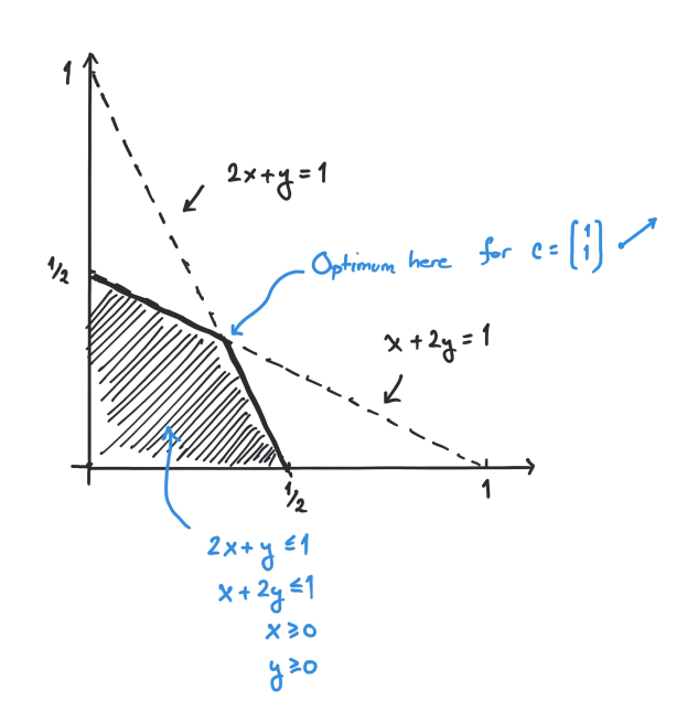

Constraints pictured as shaded area above. Optimum occurs in a vertex (corner).

We will give a general (but rather slow) algorithm below for solving linear optimization problems. In fact it all boils down to solving systems of linear inequalities. Sometimes linear optimization is referred to as linear programming. The basic theory of linear programming was pioneered, among others, by one of the inventors of the modern computer, John von Neumann.

John von Neumann (1903-1957). Picture from LANL.

Sage has much more advanced algorithms built in for solving (integer) linear optimization problems. I have translated the linear optimization problem in Example 4.31 into Sage below.

Mentimeter

Concrete LP

4.5 Fourier-Motzkin elimination

Fourier-Motzkin elimination is a classical method (dating back to 1826) for solving linear inequalities. It is also a key ingredient in an algorithm for solving linear optimization problems.

I am convinced that the best way to explain this method is by way of an extended example. For more formalities you may consult Chapter 1 of my book Undergraduate Convexity.

Consider the linear optimization problem

$\begin{array}{llrrrr} \text{Maximize} &x + y\\ \text{with constraints}\\ &2 x &+ &y &\leq &6\\ &x &+ &2 y &\leq &6\\ &x &+ &2 y &\geq &2\\ &x && &\geq &0\\ &&&y &\geq &0. \end{array} \tag{4.10}$

We might as well write this as

$\begin{array}{llrrrl} \text{Maximize} &z\\ \text{with constraints}\\ &&& z &= &x + y\\ &2 x &+ &y &\leq &6\\ &x &+ &2 y &\leq &6\\ &x &+ &2 y &\geq &2\\ &x &&&\geq &0\\ &&&y &\geq &0 \end{array}$

by adding the extra variable $z$ . This enables us to reformulate the problem as follows: Find the maximal value of $z$ , such that there exists $(x, y)\in \mathbb{R}^2$ with

$(x, y, z)\in P,$ where $P\subseteq \mathbb{R}^3$ is the set of solutions to the system

$\begin{array}{llrrrl} &&& z &= &x + y\\ &2 x &+ &y &\leq &6\\ &x &+ &2 y &\leq &6\\ &x &+ &2 y &\geq &2\\ &x &&&\geq &0\\ &&&y &\geq &0 \end{array} \tag{4.11}$

of inequalitiesAn equality $a = b$ is logically equivalent to the two inequalities $a\leq b$ and $a \geq b$ in the sense that $(a\leq b) \wedge (a\geq b) \iff a = b$ ..

We have the Gauss elimination method for solving systems of linear equations. How do we now solve (4.11), where we also have inequalities?

Well, at first we can actually do a Gauss elimination step by eliminating $x$ in the equation $z = x + y$ i.e., by putting $x = z - y$ . This is then inserted into the inequalities in (4.11):

$\begin{array}{llrrrl} &2 (z - y) &+ &y &\leq &6\\ &(z - y) &+ &2 y &\leq &6\\ &(z - y) &+ &2 y &\geq &2\\ &(z - y) & & &\geq &0\\ & & & y &\geq &0 \end{array}$

and we get the system

$\begin{array}{llrrrl} &2 z &- &y&\leq &6\\ &z &+ &y &\leq &6\\ &z &+ & y &\geq &2\\ &z &- &y &\geq &0\\ & & &y &\geq &0 \end{array}$ of inequalities in the variables $z$ and $y$ . Now we only have inequalities left and we have to invent a trick for eliminating $y$ . Let us isolate $y$ on one side of the inequality signs $\leq$ and $\geq$ :

$\begin{array}{llrrrl} &2 z &- &6 &\leq &y\\ &6 &- &z &\geq &y\\ &2 &- &z &\leq &y\\ & & &z &\geq &y\\ &&&0 &\leq &y \end{array}$

Written a little differently this is the same as

$\begin{array}{llllllllll} &2 z &- &6&\leq &{\color{red} y} \\ &&&&&{\color{red} y} &\leq &6 &- &z\\ &2&- &z&\leq &{\color{red} y} \\ &&&&&{\color{red} y} &\leq &z\\ &&&0&\leq &{\color{red} y} \end{array} \tag{4.12}$

Now the scene is set for elimination of $y$ . Listen carefully. First the inequalities in (4.12) can be boiled down to the following two inequalities

$\begin{array}{lllll} \max(2 z - 6, 2 - z, 0) &\leq &{\color{red} y}\\ && {\color{red} y} & \leq &\min(6 - z, z) \end{array} \tag{4.13}$ by using (repeatedly) that $\max(a, b) \leq c \iff a\leq c \wedge b\leq c$ and $c\leq \min(a, b) \iff c\leq a \wedge c\leq b$ for three numbers $a, b, c\in \mathbb{R}$ .

Then, finally comes the (Fourier-Motzkin) elimination step: The existence of a solution to (4.13) is equivalent to the single inequality

$\max(2 z - 6, 2 - z, 0) \leq \min(6 - z, z). \tag{4.14}$

This single inequality can be exploded or expanded (see Exercise 4.34) into the following $6 = 3\cdot 2$ inequalities

$\begin{aligned} 2 z - 6 &\leq 6 - z\\ 2 z - 6 &\leq z\\ 2 - z &\leq 6 - z\\ 2 - z &\leq z\\ 0 &\leq 6 - z\\ 0 &\leq z. \end{aligned}$

Similarly to (4.12) we now isolate $z$ from the above inequalities:

$\begin{array}{lllll} &&{\color{red} z} &\leq &4\\ &&{\color{red} z} &\leq &6\\ 1&\leq &{\color{red} z}\\ &&{\color{red} z} &\leq &6\\ 0&\leq &{\color{red} z} \end{array}$

and find that

$\begin{array}{lllll} \max(1, 0) = 1 &\leq &{\color{red} z}\\ && {\color{red} z} & \leq &\min(4, 6) = 4. \end{array}$

Therefore the maximum in the optimization problem (4.10) is $z = x + y = 4$ . How do we now find numbers $x, y\in \mathbb{R}$ satisfying the constraints in the optimization problem (4.10) with $z = x + y = 4$ ?

This is simply done inserting first $z = 4$ in (4.13). Here you get the two inequalities $2 \leq y$ and $y\leq 2$ . Therefore $y = 2$ . Since we had $x = z - y$ from the very beginning we therefore get $x = 2$ and we have the unique solution to the optimization problem.

What is the solution if we replace Maximize with Minimize in the optimization problem (4.10)?

Prove the following:

Let $x_1, \dots, x_m, y_1, \dots, y_n\in \mathbb{R}$ be $m + n$ numbers. Then

$\max(x_1, \dots, x_m) \leq \min(y_1, \dots, y_n)$ if and only if the $m n$ inequalities

$\begin{matrix} &x_1 \leq y_1 &x_1 \leq y_2 &\dots &x_1\leq y_n\\ \\ &\vdots & \vdots &\ddots &\vdots\\ \\ &x_m \leq y_1 &x_m \leq y_2 &\dots &x_m\leq y_n \end{matrix}$ are satisfied.

The following is Exercise 1.8 from my book Undergraduate Convexity.

A vitamin pill $P$ is produced using two ingredients $M_1$ and $M_2$ . The pill needs to satisfy four constraints for the vital vitamins $V_1$ and $V_2$ . It must contain at least $6$ milligrams and at most $15$ milligrams of $V_1$ and at least $5$ milligrams and at most $12$ milligrams of $V_2$ . The ingredient $M_1$ contains $3$ milligrams of $V_1$ and $2$ milligrams of $V_2$ per gram. The ingredient $M_2$ contains $2$ milligrams of $V_1$ and $3$ milligrams of $V_2$ per gram:

$\def\arraystretch{1.5} \begin{array}{c|c|c} & V_1 & V_2\\ \hline M_1 & 3 & 2\\ \hline M_2 & 2 & 3 \end{array}$

Let $x$ denote the amount of $M_1$ and $y$ the amount of $M_2$ (measured in grams) in the production of a vitamin pill. Write down a system of linear inequalities in $x$ and $y$ describing the constraints above.

We want a vitamin pill of minimal weight satisfying the constraints. How many grams of $M_1$ and $M_2$ should we mix?

Use Fourier-Motzkin elimination to solve this problem.

Check your solution by modifying the input to the Sage code in Example 4.32 using Remark 4.6.

One may also force minimization by inserting the following option

LP = MixedIntegerLinearProgram(maximization=False, solver = "GLPK").

in Example 4.32.

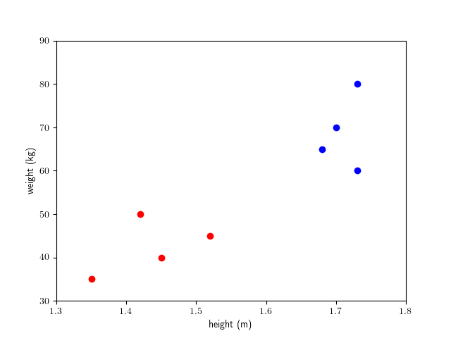
4.6 Application in machine learning and data science

To start with, consider a toy example of a machine learning problem: we wish to tell the gender of a person based on a data point consisting of the height and weight of the person.

To do this we train our model by measuring the height and weight of a lot of people. Each of these measured data points are labeled female or male according to the gender of the person.

Given a new data point, we wish to tell if the person is female or male. Here we consider a very simple model for doing this. First we need to introduce some new mathematical terms. We will introduce the terms generally for data points in $\mathbb{R}^d$ and not just in $\mathbb{R}^2$ as above.

A hyperplane in $\mathbb{R}^d$ is a generalization of a line $y = a x + b$ in the plane. In general a hyperplane is defined as the set of points $x\in \mathbb{R}^d$ satisfying

$a^\top x = b,$ where $a\in \mathbb{R}^d$ is a non-zero vector and $b$ is a number. A hyperplane divides $\mathbb{R}^d$ into two subsets: the points above or on the hyperplane satisfying $a^\top x \geq b$ and the ones below the hyperplane satisfying $a^\top x < b$ .

Suppose we are given a data set as a finite set of points in $\mathbb{R}^d$ and that each of these points are labeled with either a blue or a red color. We wish to find a hyperplane, such that the blue points are above and the red points are below the hyperplane.

We may then use the hyperplane to predict the label of a point. This could be gender, if you win or lose money buying a stock, anything with a binary classifier.

4.6.1 Formulation as a linear optimization problem

Suppose that the points labeled blue are $x_1, \dots, x_m\in \mathbb{R}^d$ and the points labeled red are $y_1, \dots, y_n\in \mathbb{R}^d$ . Then we wish to find $a\in \mathbb{R}^d$ and $b\in \mathbb{R}$ , such that

$a^\top x_i > b$ for $i = 1, \dots, m$ and

$a^\top y_j < b$ for $j = 1, \dots, n$ . One can show that these strict inequalities may be solved for $a$ and $b$ if and only if the inequalities

$\begin{aligned} a^\top x_i &\geq b + 1\\ a^\top y_j &\leq b - 1 \end{aligned}$ are solvable for $a$ and $b$ , where $i = 1, \dots, m$ and $j = 1, \dots, n$ .

It is, however, not realistic to expect data to behave this nicely. Instead one invents the rather ingenious linear optimization problem

$\begin{aligned} &\text{Minimize} &\frac{1}{m}(u_1 + \cdots + u_m) + \frac{1}{n}(v_1 + \cdots + v_n)\\ &\text{with constraints}\\ &&a^\top x_i + u_i&\geq b + 1\\ &&a^\top y_j - v_j &\leq b - 1\\ &&u_i&\geq 0\\ &&v_j&\geq 0 \end{aligned}\tag{4.15}$

for $i = 1, \dots, m$ and $j = 1, \dots, n$ . This linear optimization problem has optimal value zero if and only if data can be separated strictly. Otherwise, it finds a hyperplane minimizing the mean errors for the points involved.

The linear optimization problem (4.15) may look untied to the real world, but it has been used very successfully in the diagnosis and prognosis of breast cancer. See Mangasarian et al.

In the sage window below we have implemented the solution of the linear optimization problem (4.15), where the output is a graphical illustration of the optimal line, that separates the points in xpts and ypts with the smallest mean error as defined in the function to be minimized in (4.15).