9Convex optimization

In this last chapter we will deal exclusively with convex optimization problems.

Recall that a convex optimization problem has the form

$\begin{aligned} &\text{Minimize} &f(x_1, \dots, x_d)\\ &\text{with constraint}\\ &&(x_1, \dots, x_d)\in C, \end{aligned}$ where $C\subseteq \mathbb{R}^d$ is a convex subset (see Definition 4.18) and $f:C\rightarrow \mathbb{R}$ a convex function (see Definition 4.23). We will mainly deal with the case, where $f$ is differentiable defined on all of $\mathbb{R}^d$ in addition to just being convex defined on $C$ . Also recall that convex optimization problems are very well behaved in the sense that local minima are global (see Theorem 6.12).

Below is an example of a convex optimization problem in the plane $\mathbb{R}^2$ .

$\begin{aligned} &\text{Minimize} &x^2 + y^2\\ &\text{with constraint}\\ &&(x, y)\in C, \end{aligned}$ where $C$ is the subset of points $(x, y)$ in $\mathbb{R}^2$ satisfying

$\begin{aligned} x + y &\geq 2\\ y &\leq 2\\ x &\leq 3\\ y &\geq 1. \end{aligned}$

Sketch the subset $C$ in Example 9.1. Show that Example 9.1 really is a convex optimization problem and solve it.

Below is an example of a convex optimization problem modelling the real life problem of placing a fire station (center of circle) so that the maximal distance to the surrounding houses (points to be enclosed) is minimal.

Given $n$ points $(x_1, y_1), \dots, (x_n, y_n)\in \mathbb{R}^2$ , what is the center and radius of the smallest circle containing these points?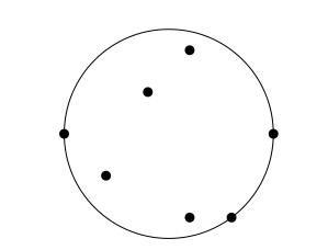

We can write this optimization problem as

$\begin{aligned} &\text{Minimize}\quad r\\ &\text{with constraint}\\ &&(x, y)\in C, \end{aligned}\tag{9.1}$ where

$C = \{(x, y)\in \mathbb{R}^2 \mid (x - x_i)^2 + (y- y_i)^2 \leq r^2\quad\text{for}\quad i = 1, \dots, n\}.$ Upon rewriting this turns into the optimization problem

$\begin{aligned} &\text{Minimize} &x^2 + y^2 + \lambda\\ &\text{with constraint}\\ &&(x, y)\in C', \end{aligned}\tag{9.2}$ where

$C' = \{(x, y, \lambda)\in \mathbb{R}^3 \mid x_i^2 + y_i^2 \leq 2 x_i x + 2 y_i y + \lambda\quad \text{for}\quad i = 1, \dots, n\}$ and $\lambda = r^2 - x^2 - y^2$ .

Prove that (9.1) and (9.2) both are convex optimization problems. Explain how (9.1) is rewritten into (9.2).

Hint

Expand

$(x - x_i)^2 + (y- y_i)^2 \leq r^2$ and put $\lambda = r^2-x^2-y^2$ .

9.1 Finding the best hyperplane separating data

In section 5.2.3 we were presented with labeled data

$(v_1, y_1), \dots, (v_m, y_m), \tag{9.3}$ where $v_i\in \mathbb{R}^d$ and $y_i = \pm 1$ . The task at hand was to separate differently labeled data by a hyperplane $\alpha^T v + \beta = 0$ , such that

$\begin{aligned} \alpha^T v_i + \beta &> 0\quad\text{if}\quad y_i = 1\\ \alpha^T v_i + \beta &< 0\quad\text{if}\quad y_i = -1 \end{aligned}\tag{9.4}$ for $i = 1, ,\dots, m$ . Please browse back to section 4.6 for the definition of a hyperplane in $\mathbb{R}^d$ .

To make this more real, consider the points $(1, 1), (-1, -1)$ with label $+1$ and the points $(-1, 1), (1, -1)$ with label $-1$ . Here a hyperplane satisfying (9.4) cannot exist: suppose that $\alpha = (\alpha_1, \alpha_2)^T$ . Then (9.4) is tantamount to the following inequalities

$\begin{aligned} \alpha_1 + \alpha_2 + \beta &> 0\\ -\alpha_1 - \alpha_2 + \beta &> 0\\ -\alpha_1 + \alpha_2 + \beta &< 0\\ \alpha_1 - \alpha_2 + \beta &< 0. \end{aligned}$ But these inequalities are unsolvable in $\alpha_1, \alpha_2$ and $\beta$ (why?).

If the data in (9.3) can be separated according to (9.4), we may find a hyperplane $(\alpha^*)^T x + \beta^* = 0$ , such that

$\begin{aligned} (\alpha^*)^T v_i + \beta^* &\geq 1\quad\text{if}\quad y_i = 1\\ (\alpha^*)^T v_i + \beta^* &\leq -1\quad\text{if}\quad y_i = -1. \end{aligned}\tag{9.5}$

How do you go from (9.4) to (9.5)?

Suppose that

$\begin{aligned} \alpha^T v_i + \beta &> 0\quad\text{if}\quad y_i = 1\\ \alpha^T v_i + \beta &< 0\quad\text{if}\quad y_i = -1. \end{aligned}$ Let

$\begin{aligned} N &= \min\{\alpha^T v_i + \beta \mid y_i = 1\}\\ M &= \max\{\alpha^T v_i + \beta \mid y_i = -1\}. \end{aligned}$ Show that $N > 0$ and $M < 0$ . How can $N$ and $M$ be applied in constructing $\alpha^*$ and $\beta^*$ ?

Consider

$\begin{aligned} \alpha^T v_i + \beta \geq N &> 0\quad\text{if}\quad y_i = 1\\ \alpha^T v_i + \beta \leq M &< 0\quad\text{if}\quad y_i = -1. \end{aligned}$ What is special about $m = \min(N, |M|)$ ?

What does best hyperplane mean in this setting? This is the one maximizing the width of the strip between the two labeled clusters.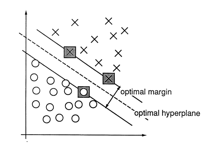

Figure from the Cortes and Vapnik paper: Support vector networks, Machine Learning, 1995.

A rather crucial insight (not explicitly mentioned in the paper by Cortes and Vapnik) is that such a hyperplane is given as $H = \{v\in \mathbb{R}^d \mid \alpha^T v + \beta\}$ satisfying (9.5) and with maximal distance to all of the data points. Therefore the function to maximize is

$\min \left\{ \frac{|\alpha^T v_i + \beta|}{|\alpha|} \middle| i = 1, \dots, m\right\}.$ This follows from the fact (see Exercise 9.7) that the distance from $H$ to a point $u$ is

$\frac{|\alpha^T u + \beta|}{|\alpha|}.$ The conditions in (9.5) may be written as $| \alpha^T v_i + \beta | \geq 1$ for $i = 1, \dots, m$ . If $m = \min\{|\alpha^T v_i + \beta| \, \mid\, i = 1, \dots, m\} > 1$ , then we may multiply $\alpha$ and $\beta$ by $1/m$ so that we may assume

$\min \left\{ \frac{|\alpha^T v_i + \beta|}{|\alpha|}\middle| i = 1, \dots, m\right\} = \frac{1}{|\alpha|}.$

The terminology support vector machines comes from the fact that $\alpha$ defines a supporting hyperplane for the two groups of points i.e., there exists $\beta_1, \beta_2\in \mathbb{R}$ such that $\alpha^T v_i + \beta_1 \geq 0$ if $y_i = 1$ with some $\alpha^T v_k + \beta_1 = 0$ for $y_k = 1$ and similarly for $y_i = -1$ with $\beta_2$ instead of $\beta_1$ and $\geq 0$ replaced by $\leq 0$ .

Let $H$ be the hyperplane in $\mathbb{R}^d$ given by $\alpha^T x + \beta = 0$ and let $v\in \mathbb{R}^d$ . The point closest to $v$ in $H$ can be found by solving the optimization problem

$\begin{aligned} &\text{Minimize} &|v - x|^2\\ &\text{with constraint}\\ &&x\in H. \end{aligned}\tag{9.6}$

Explain why (9.6) is a convex optimization problem.

Show how Theorem 7.37 can be used to solve this optimization problem by first deducing the equations

$\begin{aligned} -2(v - x) + \lambda \alpha &= 0\\ \alpha^T x + \beta &= 0 \end{aligned}\tag{9.7}$ for the Lagrange multiplier $\lambda$ . Notice here that $-2(v - x) + \lambda \alpha = 0$ above really contains $d$ equations, whereas $\alpha^T x + \beta = 0$ is only one equation in $x_1, \dots, x_d$ , where $x = (x_1, \dots, x_d)^T$ . Solve the equations (9.7) for $x\in \mathbb{R}^d$ and $\lambda\in \mathbb{R}$ . How can we be sure that $x$ really is a minimum in (9.6)?

Finally show that the distance from $H$ to $v$ is given by the formula

$\left| \frac{\alpha^T v + \beta}{|\alpha|}\right|.$

The optimal hyperplane is therefore (maximizing $1/|\alpha|$ is the same as minimizing $|\alpha|^2$ ) found by solving the convex optimization problem

$\begin{aligned} \text{Minimize}\qquad\quad &|\alpha|^2\\ \text{with constraints}&\\ \alpha^T v_i + \beta &\geq 1\quad\text{if}\quad y_i = 1\\ \alpha^T v_i + \beta &\leq -1\quad\text{if}\quad y_i = -1. \end{aligned}\tag{9.8}$

Let us explicitly write up the optimization problem (9.8) in a very simple situation: finding the best line $y = a x + b$ separating the points $(1, 1)$ and $(2, 2)$ . In the notation of (9.5), we have (without the stars on $\alpha$ and $\beta$ )

$\alpha = \begin{pmatrix} a \\ -1 \end{pmatrix}\qquad\text{and}\qquad \beta = b$ so that

$\alpha^T \begin{pmatrix} x \\ y \end{pmatrix} + b = a x - y + b = 0.$ The points are

$v_1 = \begin{pmatrix} 1 \\ 1 \end{pmatrix}\qquad\text{and}\qquad v_2 = \begin{pmatrix} 2 \\ 2 \end{pmatrix},$ where $y_1 = 1$ and $y_2 = -1$ .

Therefore (9.8) takes the form

$\begin{aligned} \text{Minimize}\qquad\quad &1 + a^2\\ \text{with constraints}&\\ a + b &\geq 2\\ 2 a + b&\leq 1 \end{aligned}\tag{9.9}$

Solve the optimization problem (9.9) and verify that the best line from the optimization problem is the one we expect it to be. Also, check how WolframAlpha solves this optimization problem.

Hint

You could maybe use Fourier-Motzkin elimination to show that

$\begin{aligned} a + b &\geq 2\\ 2 a + b&\leq 1 \end{aligned}$ implies $a \leq -1$ .

Notice that (9.8) has number of constraints equal to the number of points to be separated. For an extended (soft margin) optimization problem, when the data at hand cannot be separated we refer to section 3 of the Cortes and Vapnik paper.

Usually one does not use the optimization problem formulated in (9.8), but rather its socalled (Lagrange) dual for finding the optimal hyperplane. This dual optimization problem uses that $\alpha$ is a linear combination

$\alpha = \lambda_1 v_1 + \cdots + \lambda_m v_m \tag{9.10}$ of the support vectors. It is an optimization problem in $\Lambda^T = (\lambda_1,\dots, \lambda_m)$ from (9.10) and looks like

$\begin{aligned} \text{Maximize}\qquad\quad &\lambda_1 + \cdots + \lambda_m - \frac{1}{2} \Lambda^T D \Lambda\\ \text{with constraints}&\\ \Lambda &\geq 0\\ \Lambda^T Y &= 0, \end{aligned}\tag{9.11}$ where $Y =(y_1, \dots, y_m)^T$ is the vector of labels attached to the points $v_1, \dots, v_m$ and $D$ is the symmetric $m\times m$ matrix given by

$D_{ij} = y_i y_j\, v^T_i v_j = y_i y_j\, v_i\cdot v_j. \tag{9.12}$

The dual optimization problem (9.11) can be derived formally from the original optimization problem (9.8). This is, however, beyond the scope of this course (see section 2.1 of the Cortes and Vapnik paper).

Quadratic optimization problems, such as (9.8) can in fact be handled by Sage (well, python in this case). See CVXOPT for further information. Note that the code below needs to be executed as Python code (choose Python in the pull down). It attempts (in general) to solve the optimization problem

$\begin{aligned} \text{Minimize}\qquad\quad &\frac{1}{2} x^T Q x + p^T x\\ \text{with constraints}&\\ G x &\leq h\\ A x &= b. \end{aligned}$

In the Sage window below the optimization problem

$\begin{aligned} \text{Minimize}\qquad\quad &2 x_1^2 + x_2^2 + x_1 x_2 + x_1 + x_2\\ \text{with constraints}&\\ &x_1 \geq 0\\ &x_2 \geq 0\\ &x_1 + x_2 = 1 \end{aligned}$ has been entered.

What happens if you remove

RealNumber=float
Integer=int

from the code above?

Take a look at the input format in Example 9.10. Can you tell which optimization problem in this chapter is solved below? Also, the code below seems to report some errors after pressing the compute button. Can you make it run smoothly by making a very, very small change?

9.1.1 Separating by non-linear functions

Sometimes one needs more complex separating curves than just a line. Consider the five points

$(-1, 1), \quad (1, 1), \quad (1, -1), \quad (-1, -1),\quad \text{and} \quad (0, 0),$ where we wish to separate $(0, 0)$ from the other points. This is impossible using a line, but certainly doable by a circle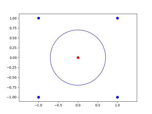

$x^2 + y^2 = r^2, \tag{9.13}$ where $0<r<\sqrt{2}$ :

The circle (9.13) may be a circle in two dimensions, but viewed in three dimensions it turns into a hyperplane in the following way.

By using the function $\varphi:\mathbb{R}^2\rightarrow \mathbb{R}^3$ given by

$\varphi(x, y) = (x^2, y^2, 1)\in \mathbb{R}^3 = \{(x_1, y_1, z_1)\mid x_1, y_1, z_1\in \mathbb{R}\},$ points lying on (9.13) map to points lying on the hyperplane in $\mathbb{R}^3$ given by

$x_1 + y_1 = r^2 z_1$ in $\mathbb{R}^3$ .

The general trick is to find a suitable map

$\varphi: \mathbb{R}^d\rightarrow \mathbb{R}^N,$ such that the transformed data

$(\varphi(x_1), y_1), \dots, (\varphi(x_m), y_m)$ becomes linearly separable. Since,

$\alpha = \lambda_1 \varphi(x_1) + \cdots + \lambda_m \varphi(x_m)$ for suitable $\lambda_1, \dots, \lambda_m\in \mathbb{R}$ , the (dual) optimization problem in (9.11) becomes

$\begin{aligned} \text{Maximize}\qquad\quad &\lambda_1 + \cdots + \lambda_m - \frac{1}{2} \Lambda^T D \Lambda\\ \text{with constraints}&\\ \Lambda &\geq 0\\ \Lambda^T Y &= 0, \end{aligned}$ where $Y =(y_1, \dots, y_m)^T$ is the vector of labels attached to the points $\varphi(x_1), \dots, \varphi(x_m)$ and $D$ is the symmetric $m\times m$ matrix given by

$D_{ij} = y_i y_j\, \varphi(x_i)\cdot \varphi(x_j). \tag{9.14}$

The beauty of the dual problem is that we do not have to care about the (sometimes astronomical, even "infinite") dimension of $\mathbb{R}^N$ . The optimization problem is situated in $\mathbb{R}^m$ , where $m$ is the number of data points (or more precisely the number of constraints). We only need a clever way of getting our hands on $\varphi(x_i)\cdot \varphi(x_j)$ in (9.14). Here an old concept from pure mathematics called kernels helps us.

9.1.2 Kernels

A kernel is a function $k: \mathbb{R}^n\times \mathbb{R}^n \rightarrow \mathbb{R}$ , that is a hidden dot product in the following sense: there exists a function

$\varphi: \mathbb{R}^n\rightarrow \mathbb{R}^N,$ such that

$k(u, v) = \varphi(u)\cdot \varphi(v). \tag{9.15}$

Let $k:\mathbb{R}^2 \times \mathbb{R}^2 \rightarrow \mathbb{R}$ be given by

$k(u, v) = (u^T v + 1)^2.$ Then

$\begin{aligned} k((x_1, y_1), (x_2, y_2)) &= (x_1 x_2 + y_1 y_2 +1)^2\\ &= x_1^2 x_2^2 + y_1^2 y_2^2 + 2 x_1 x_2 y_1 y_2 + 2 x_1 x_2 + 2 y_1 y_2 + 1. \end{aligned}\tag{9.16}$ One gleans from (9.16) that $k$ is a kernel function, since (9.15) is satisfied for $\varphi: \mathbb{R}^2\rightarrow \mathbb{R}^6$ given by

$\varphi(a, b) = (a^2, b^2, \sqrt{2} a b, \sqrt{2} a, \sqrt{2} b, 1).$

The simplest example of non-linear separation comes from the one dimensional case $\mathbb{R}$ : consider the labeled points $((-1), 1), ((1), -1), ((2), 1)$ . Show by a drawing that these points cannot be separated in $\mathbb{R}$ , but that they become separable in $\mathbb{R}^2$ by using $\varphi(x) = (x, x^2)$ i.e., that the labeled points $(\varphi(-1), 1), (\varphi(1), -1), (\varphi(2), 1)$ are linearly separable in $\mathbb{R}^2$ .

How does one glean from (9.16) that $k$ is a kernel function?

Once we have a kernel for $\varphi$ we can replace the matrix in (9.14) by

$D_{ij} = y_i y_j\, k(x_i, x_j)$

and proceed to solve the optimization problem without worrying about $\mathbb{R}^N$ (or even an infinite dimensional space).

9.1.3 The kernel perceptron algorithm

Recall the stunningly simple perceptron algorithm from section 5.2.3. This algorithm can be modified to handle non-linear separation too by using kernel functions. In fact, this modification was one of the inspirations for the development of the support vector machines described above.

After having mapped a set of vectors $x_1, \dots, x_m\in \mathbb{R}^d$ with labels $y_1, \dots, y_m\in\{\pm 1\}$ to $\varphi(x_1), \dots, \varphi(x_m)$ , via $\varphi:\mathbb{R}^d\rightarrow \mathbb{R}^N$ , we are looking for a vector $w\in \mathbb{R}^N$ , such that

$\begin{aligned} w^T \varphi(x_i) &> 0\quad\text{if}\quad y_i = 1\\ w^T \varphi(x_i) &< 0\quad\text{if}\quad y_i = -1. \end{aligned}\tag{9.17}$ Such a vector is expressible as

$w = \lambda_1 \varphi(x_1) + \cdots + \lambda_m \varphi(x_m).$ The (dual) perceptron algorithm works adjusting the coefficients $\lambda_1, \dots, \lambda_m$ successively as follows: if $w^T$ is wrong about the placement of $\varphi(x_j)$ in (9.17) i.e., if $y_j w^T \varphi(x_j) < 0$ , then let

$\lambda_j := \lambda_j + y_j.$ If we have a kernel function $k$ for $\varphi$ , then

$w^T \varphi(x_j) = w\cdot \varphi(x_j) = \sum_{i=1}^m \lambda_i \varphi(x_i)\cdot \varphi(x_j) = \sum_{i=1}^m \lambda_i k(x_i, x_j)$ and we can use the kernel function in the algorithm without resorting to computing $\varphi$ and the inner product in $\mathbb{R}^N$ .

Use the kernel function in Example 9.12 and the kernel perceptron algorithm to separate

$((-1, -1), -1), \quad ((-1, 1), -1), \quad ((1, -1), -1), \quad ((0,0), 1), \quad ((1, 1), 1).$ Sketch the points and the separating curve.

9.2 Logarithmic barrier functions

We need an algorithm for solving optimization problems like (9.8). There is a very nice trick (probably going back to von Neumann) for solving constrained optimization problems of the form

$\begin{aligned} &\text{Minimize} &f(x_1, \dots, x_n)\\ &\text{with constraint}\\ &&(x_1, \dots, x_n)\in C, \end{aligned}\tag{9.18}$ where $C$ is defined by the differentiable functions $g_i:\mathbb{R}^n\rightarrow \mathbb{R}$ as

$C = \{x\in \mathbb{R}^n \mid g_1(x) \leq 0, \dots, g_m(x)\leq 0\}.$ The functions $g_i$ define the boundary (or barrier) of $C$ . We use them to define the logarithmic barrier function

$B(x) = - \sum_{i=1}^m \log(-g_i(x))$ defined on the interior

$C^o = \{x\in \mathbb{R}^n \mid g_1(x) < 0, \dots, g_m(x) < 0\}.$ The boundary of $C$ is

$\partial C = \{x\in C \mid g_1(x) = 0 \vee \cdots \vee g_m(x) = 0\}.$ You can see that the logarithmic barrier function explodes (becomes unbounded), when a vector $x\in C^o$ approaches $\partial C$ , since $-\log(t)$ is unbounded as $t\to 0$ for $t>0$ .

The cool idea is to consider the function

$f_\epsilon(x) = f(x) + \epsilon B(x) \tag{9.19}$ for $\epsilon > 0$ . This function has a global minimum $x_\epsilon\in C^o$ .

Prove that $f_\epsilon$ is a convex function if $f$ and $g_1, \dots, g_m$ are convex functions.

Hint

Prove and use that if $f$ is a decreasing convex function (in one variable) and $g$ is a convex function, then $f(-g(x))$ is a convex function, where we assume the composition makes sense.

The upshot is that $x_\epsilon \to x_0$ as $\epsilon\to 0$ . This is the content of the following theorem, which we will not prove.

Let $x_\epsilon$ be a point in $C^o$ with

$f_\epsilon(x_\epsilon) = \min\left\{ f_\epsilon(x) \middle| x\in C^o \right\}$ for $\epsilon > 0$ and $f^* = \min\left\{ f(x) \middle| x\in C \right\}$ . Then

$0\leq f(x_\varepsilon) - f^* \leq \varepsilon m$ and $f(x_\varepsilon)\to f^*$ as $\varepsilon \to 0$ . If (9.18) has a unique optimum $x^*$ , then by using $\epsilon=\frac1n$ we obtain a sequence $x_{\frac{1}{n}}\to x^*$ as $n\to \infty$ .

We move on to give concrete examples of Theorem 9.16 in action.

9.2.1 Quadratic function with polyhedral constraints

A much used setup in optimization is minimizing a quadratic functions subject to polyhedral constraints. This is the optimization problem

$\begin{aligned} &\text{Minimize} &x^T Q x + c^T x\\ &\text{with constraint}\\ &&A x \leq b, \end{aligned}\tag{9.20}$ where $Q$ is an $n\times n$ matrix, $A$ is an $m\times n$ matrix, $c\in \mathbb{R}^n$ and $b\in \mathbb{R}^m$ .

Certainly the constraints $A x\leq b$ define a convex subset of $\mathbb{R}^n$ , but the function $x^T Q x + c^T x$ is not strictly convex unless $Q$ is positive definite. If $Q$ is not positive semidefinite (9.20) is difficult.

If $Q$ is positive semidefinite, the interior point method outlined above usually works well.

The optimization problem (9.2) has the form (9.20), when we put

$\begin{aligned} Q &= \begin{pmatrix} 1 & 0 & 0\\ 0 & 1 & 0\\ 0 & 0 & 0 \end{pmatrix}\\ c &= \begin{pmatrix} 0 \\ 0 \\ 2 \end{pmatrix}\\ A &= \begin{pmatrix} -2x_1 & -2y_1 & -1\\ \vdots & \vdots & \vdots \\ -2x_n & -2y_n & -1 \end{pmatrix}\\ b &= \begin{pmatrix} -x_1^2 - y_1^2\\ \vdots \\ -x_n^2 - y_n^2 \end{pmatrix} \end{aligned}$

The optimization problem (9.8) has the form (9.20), when we put

$\begin{aligned} Q &= \begin{pmatrix} 1 & 0 & \dots & 0 & 0\\ 0 & 1 & \dots & 0 & 0\\ \vdots & \vdots &\ddots & \vdots\\ 0 & 0 & \dots & 1 & 0\\ 0 & 0 & \dots & 0 & 0 \end{pmatrix}\\ c &= \begin{pmatrix} 0 \\ \vdots \\ 0 \end{pmatrix}\\ A &= \begin{pmatrix} -y_1 x_1 & -y_1\\ \vdots & \vdots\\ - y_n x_n & -y_n \end{pmatrix}\\ b &= \begin{pmatrix} -1\\ \vdots \\ -1 \end{pmatrix} \end{aligned}$ Here $Q$ is a $(d+1)\times (d+1)$ matrix, $A$ is an $n\times (d+1)$ matrix and $b\in \mathbb{R}^n$ .

Optimization of a quadratic function as in (9.20) is implemented below using the interior point method and exact line search. See Section 10.5.1 of my book Undergraduate Convexity for further details. Only python with numpy is used.

Below are samples of output running the interior point algorithm on the enclosing circle problem in Example 9.3.

$\epsilon = 1,\quad 0.5, \quad 0.1, \quad 0.05, \quad 0.01, \quad 0.005, \quad 0.001, \quad 0.0005, \quad 0.0001$ in the barrier function $f_\epsilon(x)$ in (9.19). We are attempting to compute the center of the smallest enclosing circle of the points

$(0, 0), \quad (2,2), \quad (-3, 2), \quad (1, 0), \quad (-2, 1), \quad (-1, 3), \quad\text{and}\quad (0, 4).$

>>> Newton(Q1, c1, A1, b1, [0,0,18], 1)
array([-0.43814179,  1.84835643,  7.69779763])
>>> Newton(Q1, c1, A1, b1, [0,0,18], 0.5)
array([-0.45244596,  1.81135335,  4.99353576])
>>> Newton(Q1, c1, A1, b1, [0,0,18], 0.1)
array([-0.49569549,  1.84020923,  2.91071666])
>>> Newton(Q1, c1, A1, b1, [0,0,18], 0.05)
array([-0.49875614,  1.87002433,  2.63917096])
>>> Newton(Q1, c1, A1, b1, [0,0,18], 0.01)
array([-0.4999099 ,  1.93327221,  2.28805064])
>>> Newton(Q1, c1, A1, b1, [0,0,18], 0.005)
array([-0.49996901,  1.95176304,  2.20331123])
>>> Newton(Q1, c1, A1, b1, [0,0,18], 0.001)
array([-0.49999729,  1.97792915,  2.09031159])
>>> Newton(Q1, c1, A1, b1, [0,0,18], 0.0005)
array([-0.49999904,  1.98432672,  2.06370265])
>>> Newton(Q1, c1, A1, b1, [0,0,18], 0.0001)
array([-0.49999991,  1.99295433,  2.0283835 ])

The first two coordinates of the output are the $x$ - and $y$ -coordinates of the center. The third is $\lambda$ from (9.2).

Try out the code in the Sage window above on the Exercises 7.48, 7.49 and 7.50. Check the output of the code by actually solving these exercises.

Compute the best line separating the labeled data

((1, 0), +1), ((2, 0), +1), ((3, 0), +1), ((3, 2), +1), ((1, 1), -1), ((2, 2), -1).

9.3 A geometric optimality criterion

Consider the general optimization problem

$\begin{aligned} &\text{Minimize} &f(x_1, \dots, x_n)\\ &\text{with constraint}\\ &&(x_1, \dots, x_n)\in C, \end{aligned}\tag{9.21}$ where $C$ is a subset of $\mathbb{R}^n$ .

Suppose that $C\subseteq \mathbb{R}^n$ is a convex subset and $f:\mathbb{R}^n\rightarrow \mathbb{R}$ a differentiable function in (9.21). If $x_0\in C$ is an optimal solution of (9.21), then

$\nabla f (x_0) (x - x_0) \geq 0\qquad\text{for every } x\in C. \tag{9.22}$ If $f$ in addition is a convex function, then (9.22) implies that $x_0$ is optimal.

Proof

If $x_0$ is an optimal solution and $x\in C\setminus\{x_0\}$ , then

$\begin{aligned} 0 &\leq f((1-t)x_0 + t x) - f(x_0) = f(x_0 + t(x-x_0)) - f(x_0)\\ &= t\,\left (\nabla f(x_0)(x-x_0) + \epsilon(t (x-x_0)) \left\vert x-x_0 \right\vert\right) \end{aligned}$ for every $t$ with $0\leq t \leq 1$ , where $\epsilon$ denotes the epsilon function in the definition of differentiability (see Definition 7.5). Therefore

$\nabla f(x_0)(x-x_0) + \epsilon(t (x-x_0)) \left\vert x-x_0 \right\vert\geq 0$ for $0\leq t\leq 1$ . This is only possible if $\nabla f(x_0)(x-x_0)\geq 0$ . We have silently applied the convexity of $C$ and the differentiability of $f$ at $x_0$ .

If $f$ in addition is convex and (9.22) holds, then Theorem 8.19 shows that $x_0$ is an optimal solution.

A nice application of Proposition 9.22 is for example to the optimization problem

$\begin{aligned} &\text{Minimize} &(x+1)^2 + (y+1)^2\\ &\text{with constraint}\\ &&x^2 + 3 y^2 \leq 1 \end{aligned}$

Here Proposition 9.22 shows that $x_0=\left(-\tfrac{1}{2}, -\tfrac{1}{2}\right)$ is optimal, since the hyperplane

$\nabla f(x_0) x = \nabla f(x_0) x_0$ touches the boundary of

$C = \{(x, y)\in \mathbb{R}^2\mid x^2 + 3y^2\leq 1\}$ as shown below.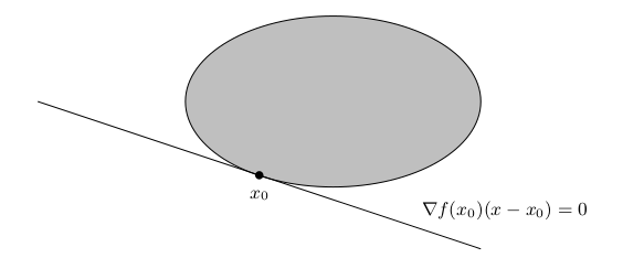

Sketch how Proposition 9.22 applies to show that an optimum in a linear programming problem

$\begin{aligned} &\text{Minimize} &c x + d y\\ &\text{with constraint}\\ &&A \begin{pmatrix} x \\ y \end{pmatrix} \leq b \end{aligned}$ in the plane $\mathbb{R}^2$ always can be found in a vertex.

Let $f:\mathbb{R}^2\rightarrow \mathbb{R}$ be a differentiable convex function and

$S =\left\{ (x, y) \middle| -1 \leq x \leq 2, -1 \leq y \leq 1 \right\}.$ Suppose that $\nabla f(x_0) = (1,0)$ for $x_0 = (-1,\frac{1}{2})$ . Prove that $x_0$ is a minimum for $f$ defined on $S$ .

Guess the solution to the optimization problem

$\min\left\{ (x-5)^2 + (y-5)^2\, \middle| \, x\geq 0,\, y\geq 0,\, x^2 + y^2 \leq 25 \right\}.$ Show that your guess was correct!

9.4 KKT

The KKT in the title of this section is short for Karush-Kuhn-Tucker.

We will limit ourselves to a convex optimization problem of the form

$\begin{aligned} &\text{Minimize} &f(x_1, \dots, x_n)\\ &\text{with constraint}\\ &&(x_1, \dots, x_n)\in C, \end{aligned}\tag{9.23}$ where $C$ is defined by the differentiable convex functions $g_i:\mathbb{R}^n\rightarrow \mathbb{R}$ for $i = 1, \dots, m$ as

$C = \{v\in \mathbb{R}^n \mid g_1(v) \leq 0, \dots, g_m(v)\leq 0\}$ and $f:\mathbb{R}^n\rightarrow \mathbb{R}$ is a convex function.

To the optimization problem (9.23) we associate the (famous) Karush-Kuhn-Tucker (KKT) conditions:

$\begin{aligned} &\lambda_1 \geq 0, \dots, \lambda_m\geq 0\\ \\ &g_1(v_0)\leq 0, \dots, g_m(v_0)\leq 0\\ \\ &\lambda_1 g_1(v_0) = 0, \dots, \lambda_m g_m(v_0) = 0\\ \\ &\nabla f(v_0) + \lambda_1 \nabla g_1(v_0) + \cdots + \lambda_m \nabla g_m(v_0) = 0. \end{aligned}\tag{9.24}$

Notice that the KKT conditions consist of $2m$ inequalities and $m+n$ equations in the $m+n$ unknowns $\lambda_1, \dots, \lambda_m, v_0 = (x_1, \dots, x_n)$ . The KKT conditions form a surprising theoretical foundation for optimization problems of the type in (9.23). You should take a peek back to the theory of Lagrange multipliers in section 7.9 and compare with (9.24).

The KKT conditions associated with the convex optimization problem in (9.1) are

$\begin{aligned} \lambda_1, \lambda_2, \lambda_3, \lambda_4 & \geq 0\\ -x -y + 2 &\leq 0\\ y - 2&\leq 0\\ x - 3&\leq 0\\ -y + 1 &\leq 0\\ \lambda_1 (- x - y + 2) &=0\\ \lambda_2 (y - 2) &= 0\\ \lambda_3 (x - 3) &= 0\\ \lambda_4 (-y + 1) &= 0\\ 2 x - \lambda_1 + \lambda_3 &= 0\\ 2 y - \lambda_1 + \lambda_2 -\lambda_4 &= 0. \end{aligned}$

Verify that the KKT conditions of the optimization problem in (9.1) are the ones given in Example 9.27.

To state our main theorem we need a definition.

The optimization problem (9.23) is called strictly feasible if there exists $z_0\in \mathbb{R}^n$ with

$\begin{aligned} g_1(z_0) &< 0\\ &\vdots\\ g_m(z_0) &< 0. \end{aligned}$

Below is the main result in our limited convex setting. We will not go into the proof, which can be found in my book Undergraduate Convexity.

Let $v_0$ be an optimal solution of (9.23). If (9.23) is strictly feasible, then the KKT conditions are satisfied at $v_0$ for suitable $\lambda_1, \dots, \lambda_m$ .
If the KKT conditions are satisfied at $z\in \mathbb{R}^n$ for some $\lambda_1, \dots, \lambda_m$ , then $z$ is an optimal solution to (9.23).

Let us now touch base with a rather simple example. Consider the optimization problem

$\begin{aligned} &\text{Minimize} &x\\ &\text{with constraint}\\ &&x\in [1, 2]. \end{aligned}\tag{9.25}$

Here $f(x) = x, g_1(x) = -x + 1$ and $g_2(x) = x - 2$ in (9.23). Therefore the KKT conditions in (9.24) are

$\begin{aligned} \lambda_1 &\geq 0\\ \lambda_2 &\geq 0\\ -x + 1 &\leq 0\\ x - 2 &\leq 0\\ \lambda_1 (- x + 1) &= 0\\ \lambda_2 (x -2 ) &= 0\\ 1 -\lambda_1 + \lambda_2 &= 0. \end{aligned}\tag{9.26}$

Before even thinking about moving on to the next section, you should attempt to find a solution $x, \lambda_1, \lambda_2$ to the above KKT conditions (inequalities) and then verify using Theorem 9.30 (ⅱ.) that $x$ is optimal. Also, try only using Theorem 9.30 (ⅰ.) and (9.26) to show that $x = 2$ is not a solution to (9.25).

Give an example of a convex optimization problem as in (9.23), which is not strictly feasible and with an optimal solution $v_0$ that does not satisfy the KKT conditions. Such an example shows that strict feasibility is necessary in Theorem 9.30 (ⅰ.).

9.5 Computing with KKT

9.5.1 Strategy

A general strategy for finding solutions to the KKT conditions in (9.24) is zooming in on (the Lagrange multipliers) $\lambda_1, \dots, \lambda_m$ testing each of them for the two cases $\lambda_i = 0$ and $\lambda_i> 0$ .

One important point, which you can read from (9.24), is that $g_i(v_0) = 0$ if $\lambda_i > 0$ . To further elaborate, if $\lambda_i > 0$ , then an optimal solution must satisfy $g_i(v_0) = 0$ .

So where exactly in (9.24) is the above claim verified?

The condition $\lambda_i = 0$ simplifies the equations

$\nabla f(v_0) + \lambda_1 \nabla g_1(v_0) + \cdots + \lambda_m \nabla g_m(v_0) = 0$ in (9.24).

In principle to solve the KKT conditions, one has to try out all the $2^m$ possibilities coming from $\lambda_i = 0$ or $\lambda_i > 0$ for $i=1, \dots, m$ .

Why $2^m$ possibilities above?

How do you solve the optimization problem (or decide there is no solution) if $\lambda_1 = \cdots = \lambda_m = 0$ ?

9.5.2 Example

Let $C$ denote the set (see Figure 9.35) of points $(x, y)\in \mathbb{R}^2$ with

$\begin{aligned} x^2 + 2y^2 &\leq 1\\ x + y &\leq 1\\ y &\leq x. \end{aligned}$ We will illustrate the mechanics of solving the KKT conditions in finding an optimal solution for

$\begin{aligned} &\text{Minimize} &x + 3 y\\ &\text{with constraint}\\ &&(x, y)\in C. \end{aligned}\tag{9.27}$

The convex set $C$ with optimal solution for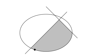 (9.27) marked.

Putting

$\begin{aligned} g_1(x, y) &= x^2 + 2 y^2 -1\\ g_2(x, y) &= x + y - 1\\ g_3(x, y) &= y - x \end{aligned}$ and $f(x, y) = x + 3y$ , we are in a position to apply Theorem 9.30, since $g_1, g_2, g_3$ are convex functions and $g_1(z_0) < 0, g_2(z_0)<0, g_3(z_0)<0$ for $z_0 = (0, -\frac{1}{2})$ . This means that an optimal solution of (9.27) satisfies the KKT conditions. The same theorem tells us that the $x_0$ in a solution of the KKT conditions is an optimal solution (here we also use that $f$ is a convex function). The full set of KKT conditions in $x, y, \lambda_1, \lambda_2, \lambda_3\in \mathbb{R}$ are

$\begin{aligned} x^2 + 2y^2 -1 &\leq 0\\ x + y -1&\leq 0\\ y - x&\leq 0\\ \lambda_1, \lambda_2, \lambda_3 & \geq 0\\ \lambda_1 (x^2 + 2y^2 -1) &=0\\ \lambda_2 (x+y -1) &= 0\\ \lambda_3 (-x + y) &= 0\\ 1 + 2 \lambda_1 x + \lambda_2 - \lambda_3 &= 0\\ 3 + 4\lambda_1 y + \lambda_2 +\lambda_3 &= 0. \end{aligned}$ A strategy for finding a solution to the KKT conditions is trying (the eight) different combinations of strict inequalities in $\lambda_1, \lambda_2, \lambda_3\geq 0$ . You can see from the last two equations that $\lambda_1 = 0$ is impossible. The condition $\lambda_1 > 0$ shows that an optimal solution has to occur on the lower arc in Figure 9.35. If $\lambda_3 > 0$ , then $x = y$ and $\lambda_2 = 1+3 \lambda_3 > 0$ by the last two equations. This implies $x = y = \frac{1}{2}$ violating $x^2 + 2 y^2 - 1 = 0$ . Therefore $\lambda_3 = 0$ . If $\lambda_2 > 0$ , then $y=1-x$ and $5 + 4 \lambda_1 + 3 \lambda_2 = 0$ by $\lambda_3 = 0$ and the last two equations. Therefore $\lambda_2=0$ . So we are left with the case $\lambda_1 > 0$ and $\lambda_2 = \lambda_3 = 0$ giving

$x = -\frac{1}{2\lambda_1}\quad\text{and}\quad y = -\frac{3}{4 \lambda_1}.$ Inserting this into $x^2 + 2 y^2 - 1 = 0$ we end up with (see Figure 9.35)

$\lambda_1 = \frac{\sqrt{11}}{2 \sqrt{2}},\quad x = -\sqrt{\frac{2}{11}} \quad\text{and}\quad y = -\frac{3}{\sqrt{22}}.$

Theorem 9.30 is beautiful mathematics. Going through the KKT conditions as above can be quite lengthy if not impossible in practice. As we have seen, there are other methods for (at least) approximating an optimal solution.

9.6 Optimization exercises

Below are some exercises especially related to the KKT conditions. In some of the exercises the minimization problem

$\begin{aligned} &\text{Minimize} &f(x_1, \dots, x_n)\\ &\text{with constraint}\\ &&(x_1, \dots, x_n)\in C, \end{aligned}\tag{9.28}$ is denoted

$\min\{f(x_1, \dots, x_n) \mid (x_1, \dots, x_n)\in C\}.$ This should cause no confusion.

Consider the optimization problem

$\begin{aligned} &\text{Minimize} &-x + y\\ &\text{with constraints}\\ &&x^2 +y^2 &\leq 1\\ &&(x+1)^2 + (y-1)^2&\leq 1 \end{aligned}\tag{9.29}$

Show that (9.29) is a convex optimization problem.
Sketch the set of constraints in $\mathbb{R}^2$ and show that $\left(-\frac{1}{2}, \frac{1}{2}\right)$ cannot be an optimal solution to (9.29).
Write up the KKT conditions for (9.29) and explain theoretically (without actually solving them) why they must have a solution.
Now solve (9.29). Is the solution unique?

Consider the function $f:\mathbb{R}^3\rightarrow \mathbb{R}$ given by

$f(x_1, x_2, x_3) = 2 x_1^2 + 3 x_2^2 + 4 x_3^2.$

Show that $f$ is strictly convex.
Let $S \subseteq \mathbb{R}^3$ denote the subset of points $(x_1, x_2, x_3)\in \mathbb{R}^3$ satisfying
$\begin{aligned} x_1 + x_2 + x_3 &\geq 1\\ x_1 + 2 x_2 + 3 x_3 &\leq 5 \end{aligned}$ Show that $S$ is a closed convex subset.
Solve the optimization problem
$\begin{aligned} &\text{Minimize} &f(x_1, x_2, x_3)\\ &\text{with constraints}\\ &&(x_1, x_2, x_3)\in S \end{aligned}\tag{9.30}$

Let $S\subseteq B \subseteq \mathbb{R}^3$ , where

$\begin{aligned} S &= \{(x, y, z)\in \mathbb{R}^3 \mid x^2 + y^2 + z^2 = 1\}\qquad\text{and}\\ B &= \{(x, y, z)\in \mathbb{R}^3 \mid x^2 + y^2 + z^2 \leq 1\}. \end{aligned}$

Why does the optimization problem
$\begin{aligned} &\text{Minimize} &x + 2y + z\\ &\text{with constraints}\\ &&(x, y, z)\in S \end{aligned}\tag{9.31}$ have a solution?
Find all optimal solutions to (9.31).
Let $a, b, c\in \mathbb{R}$ , where at least one of $a, b, c$ is non-zero. Show that an optimal solution to
$\begin{aligned} &\text{Minimize} &a x + b y + c z\\ &\text{with constraints}\\ &&(x, y, z)\in B \end{aligned}$ belongs to $S$ .

Let

$S = \left\{ (x, y)\in \mathbb{R}^2 \middle| \begin{matrix} -x & - & y & \leq & 0 \\ 2 x & - & y & \leq & 1 \\ -x & + & 2 y & \leq & 1 \end{matrix} \right\}.$

Use the KKT conditions to solve the minimization problem
$\min\left\{ -x - 4 y \middle| (x, y)\in S \right\}.$
Use the KKT conditions to solve the minimization problem
$\min\left\{ x + y \middle| (x, y)\in S \right\}.$

Solve the optimization problem

$\min\left\{ x^2 + 2 y^2 + 3 z^2- 2 x z - x y \middle| \begin{matrix} 2x^2 + y^2 + z^2 & \leq & 4 \\ 1 & \geq & x+y+z \end{matrix} \right\}.$

Let $S =\left\{ (x, y) \middle| 2 x^2 + y^2 \leq 3, \, x^2 + 2y^2 \leq 3 \right\}$ and $f(x, y) = (x-4)^2 + (y-4)^2$ .

State the KKT conditions for $\min\left\{ f(x, y) \middle| (x, y)\in S \right\}$ for $(x, y) = (1,1)$ .
Suppose now that $g(x, y) = (x-a)^2 + (y-b)^2$ . For which $a$ and $b$ does $\min\left\{ g(x, y) \middle| (x, y)\in S \right\}$ have optimum in $(1,1)$ ? State the KKT conditions when $(a, b) = (1,1)$ .

Let $f:\mathbb{R}^2\rightarrow \mathbb{R}$ be given by

$f(x, y) = (x-1)^2+ (y-1)^2 + 2 x y.$

Show that $f$ is a convex function.
Find $\min\left\{ f(x, y) \middle| (x, y)\in \mathbb{R}^2 \right\}$ . Is this minimum unique? Is $f$ a strictly convex function.
Let
$S = \left\{ (x, y)\in \mathbb{R}^2 \middle| x + y \leq 0, \quad x - y \leq 0 \right\}.$
Apply the KKT-conditions to decide if $(-1, -1)$ is an optimal solution to
$\min\left\{ f(x, y) \middle| (x, y)\in S \right\}.$
Find
$m = \min\left\{ f(x, y) \middle| (x, y)\in S \right\}$ and
$\left\{ (x, y)\in \mathbb{R}^2 \middle| f(x, y) = m \right\}.$

Let $f:\mathbb{R}^2\rightarrow \mathbb{R}$ be given by

$f(x, y) = x^2 + y^2 - e^{x-y-1}$ and let

$C =\left\{ (x, y) \middle| x - y \leq 0 \right\}.$

Show that $f:\mathbb{R}^2\rightarrow \mathbb{R}$ is not a convex function.
Show that $f$ is a convex function on the open subset
$\left\{ (x, y) \in \mathbb{R}^2 \middle| x - y< \tfrac{1}{2} \right\}$ and conclude that $f$ is convex on $C$ .
Show that $v = (0,0)$ is an optimal solution for the optimization problem $\min\left\{ f(v) \middle| v\in C \right\}$ . Is $v$ a unique optimal solution here?

Let $f:\mathbb{R}^4\rightarrow \mathbb{R}$ be given by

$f(x_1, x_2, x_3, x_4) = (x_1 - x_3)^2 + (x_2 - x_4)^2$ and $C\subseteq \mathbb{R}^4$ by

$C =\left\{ (x_1, x_2, x_3, x_4)\in \mathbb{R}^4 \middle| x_1^2 + (x_2 - 2)^2 \leq 1,\, x_3 -x_4\geq 0 \right\}.$

Show that $f$ is a convex function. Is $f$ strictly convex?
Show that $C$ is a convex subset of $\mathbb{R}^4$ .
Does there exist an optimal point $v = (x_1, x_2, x_3, x_4)\in \mathbb{R}^4$ for the minimization problem
$\min_{v\in C} f(v)$ with $x_3 = x_4 = 0$ ?
Does there exist an optimal point $v = (x_1, x_2, x_3, x_4)\in \mathbb{R}^4$ for the minimization problem
$\min_{v\in C} f(v)$ with $x_3 = x_4 = 1$ ?

Let

$f(x, y) = (x-1)^2 + y^2$ and

$C =\left\{ (x, y)\in \mathbb{R}^2 \middle| -1\leq x \leq 0,\,\, -1 \leq y \leq 1 \right\}.$ Solve the optimization problem

$\min\left\{ f(x, y) \middle| (x, y)\in C \right\}.$

Let $f:\mathbb{R}^2\rightarrow \mathbb{R}$ be given by

$f(x, y) = \tfrac{1}{2} x^2+ y^2-2 y+2.$ Below, the minimization problem

$\min\left\{ f(x, y) \middle| (x, y) \in S \right\} \tag{9.32}$ is analyzed for various subsets $S\subseteq \mathbb{R}^2$ .

Show that $f$ is a convex function
Let
$S =\left\{ (x, y)\in \mathbb{R}^2 \middle| - x + 2y \leq 1 \right\}.$ Show that $(-1, 0)\in S$ cannot be an optimal solution to (9.32). Find an optimal solution to (9.32).
Find an optimal solution in (9.32) for
$S =\left\{ (x, y)\in \mathbb{R}^2 \middle| -x + 2y \geq 1 \right\}.$
Are the optimal solutions in (2.) and (3.) unique?

Let $f:\mathbb{R}^2\rightarrow \mathbb{R}$ be given by

$f(x, y) = 2x^2 +3 x + y^2 + y.$

Show that $f$ is a convex function and solve the minimization problem $\min\left\{ f(x, y) \middle| x, y\in \mathbb{R} \right\}$ .
Now let
$S = \left\{ (x, y)\in \mathbb{R}^2 \middle| \begin{matrix} x^2 + (y+1)^2 & \leq & 1 \\ y - x & \leq & 0 \end{matrix} \right\}$ and consider the minimization problem (P) given by
$\min\left\{ f(x, y) \middle| (x, y)\in S \right\}.$
Show using the KKT conditions that $(0,0)$ is not optimal for (P).
Find an optimal solution for (P). Is it unique?