8The Hessian

In Chapter 6 we exploited the second derivative

f''(x)

of a one variable real function

f:(a, b) \rightarrow \mathbb{R}

to analyze convexity along with local minima and maxima.

In this chapter we introduce an analogue of the second derivative for real functions

f:\mathbb{R}^n\rightarrow \mathbb{R}

of several variables. This will be an

n\times n

matrix. The important notion of a matrix being positive (semi-) definite introduced in Section 3.7 will now make its appearance.

8.1 Introduction

In Section 6.4 the Taylor expansion for a one variable differentiable function

f:\mathbb{R}\rightarrow \mathbb{R}

centered a

x_0

with step size

h = x - x_0

was introduced as

f(x_0 + h) = f(x_0) + f'(x_0) h + \frac{1}{2!} f''(x_0) h^2 + \cdots \tag{8.1}

Recall that the second derivative

f''(x_0)

contains a wealth of information about the function. Especially if

f'(x_0) = 0

, then we might glean from

f''(x_0)

x_0

is a local maximum or minimum or none of these (see Theorem 6.43

and review Exercise 6.46

We also noticed that gradient descent did not work so well only descending along the gradient. We need to take the second derivative into account to get a more detailed picture of the function.

8.2 Several variables

Our main character is a differentiable function

F:\mathbb{R}^n\rightarrow \mathbb{R}

in several variables. We already know that

F(x_0 + h) = F(x_0) + \nabla F(x_0) h + \epsilon(h) \left\vert h \right\vert,

where

x_0

and

h

are vectors in

\mathbb{R}^n

(as opposed to the good old numbers in (8.1)

f(x_0 + h) = f(x_0) + f'(x_0) h + \frac{1}{2!} f''(x_0) h^2 + \cdots \tag{8.1}

). Take a look back at Definition 7.5

for the general definition of differentiability.

We wish to have an analogue of the Taylor expansion in (8.1)

f(x_0 + h) = f(x_0) + f'(x_0) h + \frac{1}{2!} f''(x_0) h^2 + \cdots \tag{8.1}

for such a function of several variables. To this end we introduce the function

g:\mathbb{R}\rightarrow \mathbb{R}

given by

g(t) = F(x_0 + t h). \tag{8.2}

Notice that

g(t) = (F\circ A)(t),

where

A: \mathbb{R}\rightarrow \mathbb{R}^n

is the function given by

A(t) = x_0 + t h

. In particular we get

g'(t) = F'(x_0 + t h) h = \nabla F(x_0 + t h) h \tag{8.3}

by using the chain rule (see Theorem 7.24

Explain how the chain rule is applied to get (8.3)

g'(t) = F'(x_0 + t h) h = \nabla F(x_0 + t h) h \tag{8.3}

The derivative

g'(t)

is also composed of several functions and again we may compute

g''(t)

by using the chain rule:

\begin{aligned} g''(t) &= (C\circ B \circ A)'(t)\\ &= (C\circ B)'(A(t)) A'(t) \\ &= C'(B(A(t))) B'(A(t)) A'(t), \end{aligned}\tag{8.4}

where

B: \mathbb{R}^n\rightarrow \mathbb{R}^n

is defined by

B(v) = \nabla F(v)^T

and

C:\mathbb{R}^n \rightarrow \mathbb{R}

C(v) = v^T h.

The Hessian matrix of

F

at the point

x\in \mathbb{R}^n

is defined by

\nabla^2 F(x) := \begin{pmatrix} \dfrac{ \partial^2 F}{ \partial x_1 \partial x_1}(x) & \cdots & \dfrac{ \partial^2 F}{ \partial x_1 \partial x_n}(x) \\ \vdots & \ddots & \vdots \\ \dfrac{ \partial^2 F}{ \partial x_n \partial x_1}(x) & \cdots & \dfrac{\partial^2 F}{ \partial x_n\partial x_n}(x) \end{pmatrix} .

A very important observation is that

\nabla^2 F(x)

above is a symmetric matrix. Again, you should review what this means by clicking back to Section 3.7.

Why is the Hessian matrix symmetric?

Suppose that

f: \mathbb{R}^2\rightarrow \mathbb{R}

is given by

f(x, y) = \sin(x y) + x^2 y^2 + y.

Then the gradient

\nabla f = \left(\frac{\partial f}{\partial x}, \frac{\partial f}{\partial y} \right)

and the Hessian

\nabla^2 f = \begin{pmatrix} \dfrac{\partial^2 f}{\partial x^2} & \dfrac{\partial^2 f}{\partial x \partial y} \\ \\ \dfrac{\partial^2 f}{\partial y \partial x} & \dfrac{\partial^2 f}{\partial y^2} \end{pmatrix}

f

are computed in the Sage window below.

xxxxxxxxxx
 
x, y = var('x, y')
f = sin(x*y) + x^2*y^2 + y
print("gradient = ", f.gradient())
print("Hessian = ", f.hessian())

Language:

See the further documentation for Calculus functions in Sage.

Verify (just this once) by hand the computations done by Sage in Example 8.4

Suppose that

f: \mathbb{R}^2\rightarrow \mathbb{R}

is given by

f(x, y) = \sin(x y) + x^2 y^2 + y.

Then the gradient

\nabla f = \left(\frac{\partial f}{\partial x}, \frac{\partial f}{\partial y} \right)

and the Hessian

\nabla^2 f = \begin{pmatrix} \dfrac{\partial^2 f}{\partial x^2} & \dfrac{\partial^2 f}{\partial x \partial y} \\ \\ \dfrac{\partial^2 f}{\partial y \partial x} & \dfrac{\partial^2 f}{\partial y^2} \end{pmatrix}

f

are computed in the Sage window below.

xxxxxxxxxx
 
x, y = var('x, y')
f = sin(x*y) + x^2*y^2 + y
print("gradient = ", f.gradient())
print("Hessian = ", f.hessian())

Language:

See the further documentation for Calculus functions in Sage.

Also, experiment with a few other functions in the Sage window and compute their Hessians.

By applying Proposition 7.11

it is not too hard to see that the Hessian matrix fits nicely into the framework above, since

B'(v) = \nabla^2 F(v). \tag{8.5}

The full application of the chain rule then gives

g''(t) = h^T \nabla^2 F(x_0 + t h) h. \tag{8.6}

Give a detailed explanation as to why (8.5)

B'(v) = \nabla^2 F(v). \tag{8.5}

holds.

8.3 Newton's method for finding critical points

We may use Newton's method for computing critical points for a function

F:\mathbb{R}^n\rightarrow \mathbb{R}

of several variables. Recall that a critical point is a point

x_0\in \mathbb{R}^n

with

\nabla F(x_0) = 0

. By (7.8)

and (8.5)

B'(v) = \nabla^2 F(v). \tag{8.5}

the computation in Newton's method becomes

x_1 = x_0 - \left(\nabla^2 F(x_0)\right)^{-1} \nabla F(x_0). \tag{8.7}

In practice the (inverse) Hessian appearing in (8.7)

x_1 = x_0 - \left(\nabla^2 F(x_0)\right)^{-1} \nabla F(x_0). \tag{8.7}

is often a heavy computational burden. This leads to the socalled quasi-Newton methods, where the inverse Hessian in (8.7)

x_1 = x_0 - \left(\nabla^2 F(x_0)\right)^{-1} \nabla F(x_0). \tag{8.7}

is replaced by other matrices.

We will return to the logistic regression in Example 7.34

about the Challenger disaster. Here we sought to maximize the function

\ell(\alpha, \beta) = \sum_{i=1}^m E_i (\alpha + \beta x_i) - \log(1 + e^{\alpha + \beta x_i}). \tag{8.8}

In order to employ Newton's method we compute the gradient and the Hessian of (8.8)

\ell(\alpha, \beta) = \sum_{i=1}^m E_i (\alpha + \beta x_i) - \log(1 + e^{\alpha + \beta x_i}). \tag{8.8}

\begin{aligned} \frac{\partial \ell}{\partial \alpha} &= \sum_{i=1}^m E_i - \sigma(\alpha + \beta x_i)\\ \frac{\partial \ell}{\partial \beta} &= \sum_{i=1}^m E_i x_i - x_ i\sigma(\alpha + \beta x_i)\\ \frac{\partial^2 \ell}{\partial \alpha^2} &= \sum_{i=1}^m - \sigma'(\alpha + \beta x_i)\\ \frac{\partial^2 \ell}{\partial \beta \partial \alpha} &= \sum_{i=1}^m -\sigma'(\alpha + \beta x_i) x_i\\ \frac{\partial^2 \ell}{\partial \beta^2} &= \sum_{i=1}^m - \sigma'(\alpha + \beta x_i) x_i^2, \end{aligned}\tag{8.9}

where

\sigma(t) = \frac{1}{1 + e^{-t}}

is the sigmoid function.

Notice the potential problem in using Newton's method here: the formula for the second order derivatives in (8.9)

\begin{aligned} \frac{\partial \ell}{\partial \alpha} &= \sum_{i=1}^m E_i - \sigma(\alpha + \beta x_i)\\ \frac{\partial \ell}{\partial \beta} &= \sum_{i=1}^m E_i x_i - x_ i\sigma(\alpha + \beta x_i)\\ \frac{\partial^2 \ell}{\partial \alpha^2} &= \sum_{i=1}^m - \sigma'(\alpha + \beta x_i)\\ \frac{\partial^2 \ell}{\partial \beta \partial \alpha} &= \sum_{i=1}^m -\sigma'(\alpha + \beta x_i) x_i\\ \frac{\partial^2 \ell}{\partial \beta^2} &= \sum_{i=1}^m - \sigma'(\alpha + \beta x_i) x_i^2, \end{aligned}\tag{8.9}

show that if the

\alpha +\beta x_i

are just mildly big, say

\geq 50

, then the Hessian is extremely close to the zero matrix and therefore Sage considers it non-invertible and (8.7)

x_1 = x_0 - \left(\nabla^2 F(x_0)\right)^{-1} \nabla F(x_0). \tag{8.7}

fails.

In the code below we have nudged the initial vector so that it works, but you can easily set other values and see its failure. Optimization is not just mathematics, it also calls for some good (engineering) implementation skills (see for example details on the quasi Newton algorithms).

In the instance below we do, however, get a gradient that is practically

(0, 0)

Code for Newton's method

xxxxxxxxxx
 
x0 = [11,-0.2] 
noofits = 10
  
​
x = [53.0, 56.0, 57.0, 63.0, 66.0, 67.0, 67.0, 67.0, 68.0, 69.0, 70.0, 70.0, 70.0, 70.0, 72.0, 73.0, 75.0, 75.0, 76.0, 76.0, 78.0, 79.0, 80.0, 81.0]
E = [1.0, 1.0, 1.0, 0.0, 0.0, 0.0, 0.0, 0.0, 0.0, 0.0, 0.0, 1.0, 0.0, 1.0, 0.0, 0.0, 0.0, 1.0, 0.0, 0.0, 0.0, 0.0, 0.0, 0.0]
​
Es = sum(E)
Exs = sum(u*v for (u, v) in zip(x, E))
    
def sigmoid(a, b, x):
  s = 1/(1 + exp(-a - b*x))
  return s.n()
​
def sigmoidm(a, b, x):
  s = sigmoid(a, b, x)
  return s*(1-s)
      
def gradient(v):
  a = v[0]
  b = v[1]
  return vector((Es - sum(sigmoid(a, b, t) for t in x), Exs - sum(t*sigmoid(a, b, t) for t in x)))
    
def hessian(v):
  a = v[0]
  b = v[1]
  h11 = - sum(sigmoidm(a, b, t) for t in x)
  h12 = - sum(sigmoidm(a, b, t)*t for t in x)
  h22 = - sum(sigmoidm(a, b, t)*t*t for t in x)
  return matrix([[h11, h12], [h12, h22]])
​
def newtonstep(v0):
  d = gradient(v0)
  h = hessian(v0)
  return v0 - h.inverse()*d
​
v = vector(x0)  
for k in range(noofits):
  print(v)
  v = newtonstep(v)
​
print("x0 = ", x0)
print("Number of Newton iterations =  ", noofits)
print("Predicted maximal point =  ", v)
​
alpha = v[0]
beta = v[1]
​
print("Gradient at predicted maximal point = ", gradient(v))
print("Predicted probability of failure at 31F = ", sigmoid(alpha, beta, 31))

Language:

8.3.1 Transforming data for better numerical performance

The numerical problems with Newton's method in Example 8.7

We will return to the logistic regression in Example 7.34

about the Challenger disaster. Here we sought to maximize the function

\ell(\alpha, \beta) = \sum_{i=1}^m E_i (\alpha + \beta x_i) - \log(1 + e^{\alpha + \beta x_i}). \tag{8.8}

In order to employ Newton's method we compute the gradient and the Hessian of (8.8)

\ell(\alpha, \beta) = \sum_{i=1}^m E_i (\alpha + \beta x_i) - \log(1 + e^{\alpha + \beta x_i}). \tag{8.8}

\begin{aligned} \frac{\partial \ell}{\partial \alpha} &= \sum_{i=1}^m E_i - \sigma(\alpha + \beta x_i)\\ \frac{\partial \ell}{\partial \beta} &= \sum_{i=1}^m E_i x_i - x_ i\sigma(\alpha + \beta x_i)\\ \frac{\partial^2 \ell}{\partial \alpha^2} &= \sum_{i=1}^m - \sigma'(\alpha + \beta x_i)\\ \frac{\partial^2 \ell}{\partial \beta \partial \alpha} &= \sum_{i=1}^m -\sigma'(\alpha + \beta x_i) x_i\\ \frac{\partial^2 \ell}{\partial \beta^2} &= \sum_{i=1}^m - \sigma'(\alpha + \beta x_i) x_i^2, \end{aligned}\tag{8.9}

where

\sigma(t) = \frac{1}{1 + e^{-t}}

is the sigmoid function.

Notice the potential problem in using Newton's method here: the formula for the second order derivatives in (8.9)

\begin{aligned} \frac{\partial \ell}{\partial \alpha} &= \sum_{i=1}^m E_i - \sigma(\alpha + \beta x_i)\\ \frac{\partial \ell}{\partial \beta} &= \sum_{i=1}^m E_i x_i - x_ i\sigma(\alpha + \beta x_i)\\ \frac{\partial^2 \ell}{\partial \alpha^2} &= \sum_{i=1}^m - \sigma'(\alpha + \beta x_i)\\ \frac{\partial^2 \ell}{\partial \beta \partial \alpha} &= \sum_{i=1}^m -\sigma'(\alpha + \beta x_i) x_i\\ \frac{\partial^2 \ell}{\partial \beta^2} &= \sum_{i=1}^m - \sigma'(\alpha + \beta x_i) x_i^2, \end{aligned}\tag{8.9}

show that if the

\alpha +\beta x_i

are just mildly big, say

\geq 50

, then the Hessian is extremely close to the zero matrix and therefore Sage considers it non-invertible and (8.7)

x_1 = x_0 - \left(\nabla^2 F(x_0)\right)^{-1} \nabla F(x_0). \tag{8.7}

fails.

In the instance below we do, however, get a gradient that is practically

(0, 0)

Code for Newton's method

xxxxxxxxxx
 
x0 = [11,-0.2] 
noofits = 10
  
​
x = [53.0, 56.0, 57.0, 63.0, 66.0, 67.0, 67.0, 67.0, 68.0, 69.0, 70.0, 70.0, 70.0, 70.0, 72.0, 73.0, 75.0, 75.0, 76.0, 76.0, 78.0, 79.0, 80.0, 81.0]
E = [1.0, 1.0, 1.0, 0.0, 0.0, 0.0, 0.0, 0.0, 0.0, 0.0, 0.0, 1.0, 0.0, 1.0, 0.0, 0.0, 0.0, 1.0, 0.0, 0.0, 0.0, 0.0, 0.0, 0.0]
​
Es = sum(E)
Exs = sum(u*v for (u, v) in zip(x, E))
    
def sigmoid(a, b, x):
  s = 1/(1 + exp(-a - b*x))
  return s.n()
​
def sigmoidm(a, b, x):
  s = sigmoid(a, b, x)
  return s*(1-s)
      
def gradient(v):
  a = v[0]
  b = v[1]
  return vector((Es - sum(sigmoid(a, b, t) for t in x), Exs - sum(t*sigmoid(a, b, t) for t in x)))
    
def hessian(v):
  a = v[0]
  b = v[1]
  h11 = - sum(sigmoidm(a, b, t) for t in x)
  h12 = - sum(sigmoidm(a, b, t)*t for t in x)
  h22 = - sum(sigmoidm(a, b, t)*t*t for t in x)
  return matrix([[h11, h12], [h12, h22]])
​
def newtonstep(v0):
  d = gradient(v0)
  h = hessian(v0)
  return v0 - h.inverse()*d
​
v = vector(x0)  
for k in range(noofits):
  print(v)
  v = newtonstep(v)
​
print("x0 = ", x0)
print("Number of Newton iterations =  ", noofits)
print("Predicted maximal point =  ", v)
​
alpha = v[0]
beta = v[1]
​
print("Gradient at predicted maximal point = ", gradient(v))
print("Predicted probability of failure at 31F = ", sigmoid(alpha, beta, 31))

Language:

can be prevented by transforming the input data. It makes sense to transform data from large numbers to smaller numbers around

0

. There is a rather standard way of doing this.

Suppose in logistic regression we have a set of data

x_1, x_2, \dots, x_n \tag{8.10}

associated with outcomes

E_1, \dots, E_n

. Then the function

\ell(\alpha, \beta) = \sum_{i=1}^m E_i (\alpha + \beta x_i) - \log(1 + e^{\alpha + \beta x_i}).

from Example 7.32

becomes much more manageable if we first transform the data according to

x'_i = \frac{x_i - \overline{x}}{\sigma}

and instead optimize the function

\ell'(\alpha, \beta) = \sum_{i=1}^m E_i (\alpha + \beta x'_i) - \log(1 + e^{\alpha + \beta x'_i}).

Here

\overline{x} = \frac{x_1 + x_2 + \cdots + x_n}{n}

is the mean value and

\sigma^2 = \frac{(x_1 - \overline{x})^2 + (x_2 - \overline{x})^2 + \cdots + (x_n - \overline{x})^2}{n}

the variance of the data in (8.10)

x_1, x_2, \dots, x_n \tag{8.10}

Now if

\alpha'

and

\beta'

is an optimum for

\ell'

, then

\begin{aligned} \alpha &= \alpha' - \frac{\overline{x}}{\sigma} \beta'\\ \beta &= \frac{\beta'}{\sigma} \end{aligned}\tag{8.11}

is an optimum for

\ell

, since

\ell'(\alpha, \beta) = \ell\left(\alpha - \beta \frac{\overline{x}}{\sigma}, \frac{\beta}{\sigma}\right).

Why is the claim/trick alluded to in (8.11)

\begin{aligned} \alpha &= \alpha' - \frac{\overline{x}}{\sigma} \beta'\\ \beta &= \frac{\beta'}{\sigma} \end{aligned}\tag{8.11}

true?

Below is a snippet of Sage code implementing the trick in (8.11)

\begin{aligned} \alpha &= \alpha' - \frac{\overline{x}}{\sigma} \beta'\\ \beta &= \frac{\beta'}{\sigma} \end{aligned}\tag{8.11}

. The function test takes as input x0 (an initial vector like [0,0]) and noofits (the number of iterations of Newton's method). You execute this in the Sage window by adding for example

test([0,0], 10)

and then pressing Compute.

Experiment and compare with the official output from Example 7.34

. Also, compute the gradient of the output below for the original non-transformed problem.

Transformed code

xxxxxxxxxx
 
x = [53.0, 56.0, 57.0, 63.0, 66.0, 67.0, 67.0, 67.0, 68.0, 69.0, 70.0, 70.0, 70.0, 70.0, 72.0, 73.0, 75.0, 75.0, 76.0, 76.0, 78.0, 79.0, 80.0, 81.0]
E = [1.0, 1.0, 1.0, 0.0, 0.0, 0.0, 0.0, 0.0, 0.0, 0.0, 0.0, 1.0, 0.0, 1.0, 0.0, 0.0, 0.0, 1.0, 0.0, 0.0, 0.0, 0.0, 0.0, 0.0]
mean = sum(x)/len(x)
std = sqrt(sum(map(lambda t: (t-mean)^2, x))/len(x))
​
x = list(map(lambda t: (t-mean)/std, x))
​
​
Es = sum(E)
Exs = sum(u*v for (u, v) in zip(x, E))
    
def sigmoid(a, b, x):
  s = 1/(1 + exp(-a - b*x))
  return s.n()
​
def sigmoidm(a, b, x):
  s = sigmoid(a, b, x)
  return s*(1-s)
      
def gradient(v):
  a = v[0]
  b = v[1]
  return vector((Es - sum(sigmoid(a, b, t) for t in x), Exs - sum(t*sigmoid(a, b, t) for t in x)))
    
def hessian(v):
  a = v[0]
  b = v[1]
  h11 = - sum(sigmoidm(a, b, t) for t in x)
  h12 = - sum(sigmoidm(a, b, t)*t for t in x)
  h22 = - sum(sigmoidm(a, b, t)*t*t for t in x)
  return matrix([[h11, h12], [h12, h22]])
​
def newtonstep(v0):
  d = gradient(v0)
  h = hessian(v0)
  return v0 - h.inverse()*d
​
​
def test(x0, noofits):
  v = vector(x0)  
  for k in range(noofits):
    print(v)
    v = newtonstep(v)
  print("Number of Newton iterations =  ", noofits)
  print("Predicted maximal point in transformed problem =  ", v)
  tv =   matrix([[1, -mean/std], [0, 1/std]])*v
  print("Predicted maximal point in original problem =  ", tv)

Language:

8.4 The Taylor series in several variables

Now we are in a position to state at least the first terms in the Taylor expansion for a differentiable function

F:\mathbb{R}^n\rightarrow \mathbb{R}

. The angle of the proof is to reduce to the one-dimensional case through the function

g(t)

defined in (8.2)

g(t) = F(x_0 + t h). \tag{8.2}

. Here one may prove that

g(t) = g(0) + g'(0) t + \frac{1}{2} g''(0) t^2 + \epsilon(t)t^2, \tag{8.12}

where

\epsilon(0) = 0

with

\epsilon

continuous at

0

, much like in the definition of differentiability except that we also include the second derivative.

Now (8.12)

g(t) = g(0) + g'(0) t + \frac{1}{2} g''(0) t^2 + \epsilon(t)t^2, \tag{8.12}

translates into

F(x_0 + t h) = F(x_0) + \left(\nabla F(x_0) h \right) t + \frac{1}{2} \left( h^T \nabla^2 F(x_0) h \right) t^2 + \epsilon(t) t^2 \tag{8.13}

by using (8.3)

g'(t) = F'(x_0 + t h) h = \nabla F(x_0 + t h) h \tag{8.3}

and (8.6)

g''(t) = h^T \nabla^2 F(x_0 + t h) h. \tag{8.6}

From (8.13)

F(x_0 + t h) = F(x_0) + \left(\nabla F(x_0) h \right) t + \frac{1}{2} \left( h^T \nabla^2 F(x_0) h \right) t^2 + \epsilon(t) t^2 \tag{8.13}

one reads the following nice criterion, which may be viewed as a several variable generalization of Theorem 6.43

Let

x_0

be a critical point for

F:\mathbb{R}^n\rightarrow \mathbb{R}

. Then

$x_0$ is a local minimum if $\nabla^2 F(x_0)$ is positive definite.
$x_0$ is a local maximum if $-\nabla^2 F(x_0)$ is positive definite (here we call $\nabla^2 F(x_0)$ negative definite).
$x_0$ is a saddle point if $\nabla^2 F(x_0)$ is indefinite.

We need to clarify two things concerning the above theorem.

An $n\times n$ indefinite matrix is a symmetric matrix $A$ with the property that there exists $u, v\in \mathbb{R}^n$ with $\begin{aligned} u^T A u &>0\quad\text{and}\\ v^T A v &<0 \end{aligned}$ i.e., neither $A$ nor $-A$ is positive semidefinite.
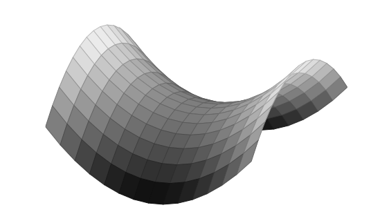
A saddle point $x_0$ for $F$ is defined by the existence of two vectors $u, v\in \mathbb{R}^n$ , such that $\begin{aligned} &t=0\quad \text{is a local minimum for the function}\quad f(t) = F(x_0 + t u)\\ &t=0\quad \text{is a local maximum for the function}\quad g(t) = F(x_0 + t v) \end{aligned}$ as illustrated in the graphics below.

Consider, with our new technology in Theorem 8.9

Let

x_0

be a critical point for

F:\mathbb{R}^n\rightarrow \mathbb{R}

. Then

$x_0$ is a local minimum if $\nabla^2 F(x_0)$ is positive definite.
$x_0$ is a local maximum if $-\nabla^2 F(x_0)$ is positive definite (here we call $\nabla^2 F(x_0)$ negative definite).
$x_0$ is a saddle point if $\nabla^2 F(x_0)$ is indefinite.

, Exercise 7.22

once again. Here we analyzed the point

v_0 = (0, 0)

for the function

f(x, y) = x^3 + x y + y^3

and showed (by a trick) that

v_0

is neither a local maximum nor a local minimum for

f

. The Hessian matrix for

f(x, y)

v_0

H = \begin{pmatrix} 0 & 1 \\ 1 & 0 \end{pmatrix}.

Now Theorem 8.9

Let

x_0

be a critical point for

F:\mathbb{R}^n\rightarrow \mathbb{R}

. Then

$x_0$ is a local minimum if $\nabla^2 F(x_0)$ is positive definite.
$x_0$ is a local maximum if $-\nabla^2 F(x_0)$ is positive definite (here we call $\nabla^2 F(x_0)$ negative definite).
$x_0$ is a saddle point if $\nabla^2 F(x_0)$ is indefinite.

(ⅲ.) shows that

v_0

is a saddle point, since

\begin{pmatrix} x & y \end{pmatrix} H \begin{pmatrix} x \\ y \end{pmatrix} = 2 x y

and

\begin{aligned} u^T H u &> 0\qquad\text{for } u = \begin{pmatrix} 1 \\ 1 \end{pmatrix}\\ v^T H v &< 0\qquad\text{for } v = \begin{pmatrix} 1 \\ -1 \end{pmatrix}. \end{aligned}

xxxxxxxxxx
 
x, y = var('x, y')
a = 1
plot3d(x^3 + a*x*y+ y^3, (x, -0.4, 0.4), (y, -0.4, 0.4), 
adaptive=True, color=rainbow(60, 'rgbtuple'))

Language:

Try plotting the graph for different values of aa=4 shows the saddle point clearly. in the Sage window in Example 8.11

Consider, with our new technology in Theorem 8.9

Let

x_0

be a critical point for

F:\mathbb{R}^n\rightarrow \mathbb{R}

. Then

$x_0$ is a local minimum if $\nabla^2 F(x_0)$ is positive definite.
$x_0$ is a local maximum if $-\nabla^2 F(x_0)$ is positive definite (here we call $\nabla^2 F(x_0)$ negative definite).
$x_0$ is a saddle point if $\nabla^2 F(x_0)$ is indefinite.

, Exercise 7.22

once again. Here we analyzed the point

v_0 = (0, 0)

for the function

f(x, y) = x^3 + x y + y^3

and showed (by a trick) that

v_0

is neither a local maximum nor a local minimum for

f

. The Hessian matrix for

f(x, y)

v_0

H = \begin{pmatrix} 0 & 1 \\ 1 & 0 \end{pmatrix}.

Now Theorem 8.9

Let

x_0

be a critical point for

F:\mathbb{R}^n\rightarrow \mathbb{R}

. Then

$x_0$ is a local minimum if $\nabla^2 F(x_0)$ is positive definite.
$x_0$ is a local maximum if $-\nabla^2 F(x_0)$ is positive definite (here we call $\nabla^2 F(x_0)$ negative definite).
$x_0$ is a saddle point if $\nabla^2 F(x_0)$ is indefinite.

(ⅲ.) shows that

v_0

is a saddle point, since

\begin{pmatrix} x & y \end{pmatrix} H \begin{pmatrix} x \\ y \end{pmatrix} = 2 x y

and

\begin{aligned} u^T H u &> 0\qquad\text{for } u = \begin{pmatrix} 1 \\ 1 \end{pmatrix}\\ v^T H v &< 0\qquad\text{for } v = \begin{pmatrix} 1 \\ -1 \end{pmatrix}. \end{aligned}

xxxxxxxxxx
 
x, y = var('x, y')
a = 1
plot3d(x^3 + a*x*y+ y^3, (x, -0.4, 0.4), (y, -0.4, 0.4), 
adaptive=True, color=rainbow(60, 'rgbtuple'))

Language:

. What do you observe for the point

v_0

with respect to the function? Does a have to be a number? Could it be a symbolic expression in the variables x and y like a = -10*cos(x)*sin(y)?

Check the computation of the Hessian matrix

H

in Example 8.11

Consider, with our new technology in Theorem 8.9

Let

x_0

be a critical point for

F:\mathbb{R}^n\rightarrow \mathbb{R}

. Then

$x_0$ is a local minimum if $\nabla^2 F(x_0)$ is positive definite.
$x_0$ is a local maximum if $-\nabla^2 F(x_0)$ is positive definite (here we call $\nabla^2 F(x_0)$ negative definite).
$x_0$ is a saddle point if $\nabla^2 F(x_0)$ is indefinite.

, Exercise 7.22

once again. Here we analyzed the point

v_0 = (0, 0)

for the function

f(x, y) = x^3 + x y + y^3

and showed (by a trick) that

v_0

is neither a local maximum nor a local minimum for

f

. The Hessian matrix for

f(x, y)

v_0

H = \begin{pmatrix} 0 & 1 \\ 1 & 0 \end{pmatrix}.

Now Theorem 8.9

Let

x_0

be a critical point for

F:\mathbb{R}^n\rightarrow \mathbb{R}

. Then

$x_0$ is a local minimum if $\nabla^2 F(x_0)$ is positive definite.
$x_0$ is a local maximum if $-\nabla^2 F(x_0)$ is positive definite (here we call $\nabla^2 F(x_0)$ negative definite).
$x_0$ is a saddle point if $\nabla^2 F(x_0)$ is indefinite.

(ⅲ.) shows that

v_0

is a saddle point, since

\begin{pmatrix} x & y \end{pmatrix} H \begin{pmatrix} x \\ y \end{pmatrix} = 2 x y

and

\begin{aligned} u^T H u &> 0\qquad\text{for } u = \begin{pmatrix} 1 \\ 1 \end{pmatrix}\\ v^T H v &< 0\qquad\text{for } v = \begin{pmatrix} 1 \\ -1 \end{pmatrix}. \end{aligned}

xxxxxxxxxx
 
x, y = var('x, y')
a = 1
plot3d(x^3 + a*x*y+ y^3, (x, -0.4, 0.4), (y, -0.4, 0.4), 
adaptive=True, color=rainbow(60, 'rgbtuple'))

Language:

by showing that the Hessian matrix for

f

at the point

(x, y)

\begin{pmatrix} 6 x & 1\\ 1 & 6 y \end{pmatrix}.

What about

u

and

v

in Example 8.11

Consider, with our new technology in Theorem 8.9

Let

x_0

be a critical point for

F:\mathbb{R}^n\rightarrow \mathbb{R}

. Then

$x_0$ is a local minimum if $\nabla^2 F(x_0)$ is positive definite.
$x_0$ is a local maximum if $-\nabla^2 F(x_0)$ is positive definite (here we call $\nabla^2 F(x_0)$ negative definite).
$x_0$ is a saddle point if $\nabla^2 F(x_0)$ is indefinite.

, Exercise 7.22

once again. Here we analyzed the point

v_0 = (0, 0)

for the function

f(x, y) = x^3 + x y + y^3

and showed (by a trick) that

v_0

is neither a local maximum nor a local minimum for

f

. The Hessian matrix for

f(x, y)

v_0

H = \begin{pmatrix} 0 & 1 \\ 1 & 0 \end{pmatrix}.

Now Theorem 8.9

Let

x_0

be a critical point for

F:\mathbb{R}^n\rightarrow \mathbb{R}

. Then

$x_0$ is a local minimum if $\nabla^2 F(x_0)$ is positive definite.
$x_0$ is a local maximum if $-\nabla^2 F(x_0)$ is positive definite (here we call $\nabla^2 F(x_0)$ negative definite).
$x_0$ is a saddle point if $\nabla^2 F(x_0)$ is indefinite.

(ⅲ.) shows that

v_0

is a saddle point, since

\begin{pmatrix} x & y \end{pmatrix} H \begin{pmatrix} x \\ y \end{pmatrix} = 2 x y

and

\begin{aligned} u^T H u &> 0\qquad\text{for } u = \begin{pmatrix} 1 \\ 1 \end{pmatrix}\\ v^T H v &< 0\qquad\text{for } v = \begin{pmatrix} 1 \\ -1 \end{pmatrix}. \end{aligned}

xxxxxxxxxx
 
x, y = var('x, y')
a = 1
plot3d(x^3 + a*x*y+ y^3, (x, -0.4, 0.4), (y, -0.4, 0.4), 
adaptive=True, color=rainbow(60, 'rgbtuple'))

Language:

? How do they relate to the hint given in Exercise 7.22

Give an example of a function

F:\mathbb{R}^2\rightarrow \mathbb{R}

having a local minimum at

x_0

, where

\nabla^2 F(x_0)

is not positive definite.

The following exercise is a sci2u exercise from the Calculus book.

The point $\left(0, \frac{\sqrt{3}}{3}\right)$ is a critical point for
$f(x, y) = x^3 + y^3 - y.$
What does Theorem 8.9
Let $x_0$ be a critical point for $F:\mathbb{R}^n\rightarrow \mathbb{R}$ . Then
1. $x_0$ is a local minimum if $\nabla^2 F(x_0)$ is positive definite.
2. $x_0$ is a local maximum if $-\nabla^2 F(x_0)$ is positive definite (here we call $\nabla^2 F(x_0)$ negative definite).
3. $x_0$ is a saddle point if $\nabla^2 F(x_0)$ is indefinite.
say about this point?
The point $\left(\frac{1}{3}, \frac{1}{3}\right)$ is a critical point for
$f(x, y) = -x^3 -x^2 + x - y^3 + 2 y^2 - y.$
What does Theorem 8.9
Let $x_0$ be a critical point for $F:\mathbb{R}^n\rightarrow \mathbb{R}$ . Then
1. $x_0$ is a local minimum if $\nabla^2 F(x_0)$ is positive definite.
2. $x_0$ is a local maximum if $-\nabla^2 F(x_0)$ is positive definite (here we call $\nabla^2 F(x_0)$ negative definite).
3. $x_0$ is a saddle point if $\nabla^2 F(x_0)$ is indefinite.
say about this point?
The point $(0, 1)$ is a critical point for
$f(x, y) = x^3 - x^2 + y^3 - y^2 - y.$
What does Theorem 8.9
Let $x_0$ be a critical point for $F:\mathbb{R}^n\rightarrow \mathbb{R}$ . Then
1. $x_0$ is a local minimum if $\nabla^2 F(x_0)$ is positive definite.
2. $x_0$ is a local maximum if $-\nabla^2 F(x_0)$ is positive definite (here we call $\nabla^2 F(x_0)$ negative definite).
3. $x_0$ is a saddle point if $\nabla^2 F(x_0)$ is indefinite.
say about this point?

Consider the function

f(x, y) = x^4 y^2 + x^2 y^4 - 3 x^2 y^2.

Compute its critical points and decide on their types according to Theorem 8.9

Let

x_0

be a critical point for

F:\mathbb{R}^n\rightarrow \mathbb{R}

. Then

$x_0$ is a local minimum if $\nabla^2 F(x_0)$ is positive definite.
$x_0$ is a local maximum if $-\nabla^2 F(x_0)$ is positive definite (here we call $\nabla^2 F(x_0)$ negative definite).
$x_0$ is a saddle point if $\nabla^2 F(x_0)$ is indefinite.

. Try to convince yourself that

f(x, y) \geq -1

for every

x, y\in \mathbb{R}

Look at the minimization problem

\min f(x, y)

subject to

(x, y)\in C = \{(x, y) \mid -M \leq x \leq M, \,\, -M \leq y \leq M\},

where

M

is a big number.

Give an example of a function

f:\mathbb{R}\rightarrow \mathbb{R}

that has a local maximum, but where there exists

x\in \mathbb{R}

with

f(x) > M

for any given (large) number

M

8.5 Convex functions of several variables

Below is the generalization of Theorem 6.53

to several variables. You have already seen this in Exercise 6.54

, right?

Let

f: U\rightarrow \mathbb{R}

be a differentiable function, where

U\subseteq \mathbb{R}^n

is an open convex subset. Then

f

is convex if and only if

f(x) \geq f(x_0) + \nabla f(x_0) (x-x_0) \tag{8.14}

for every

x, x_0\in U

Proof

Suppose that (8.14)

f(x) \geq f(x_0) + \nabla f(x_0) (x-x_0) \tag{8.14}

holds and let

x_t = (1-t)x_0 + t x

with

0 \leq t \leq 1

, where

x_0, x\in U

. To prove that

f

is convex we must verify the inequality

f(x_t) \leq (1-t) f(x_0) + t f(x). \tag{8.15}

Let

\xi = \nabla f(x_t)

. Then

\begin{aligned} f(x) &\geq f(x_t) + \xi (1-t) (x-x_0)\\ f(x_0) &\geq f(x_t) - \xi t (x-x_0) \end{aligned}

by (8.14)

f(x) \geq f(x_0) + \nabla f(x_0) (x-x_0) \tag{8.14}

. If you multiply the first inequality by

t

, the second by

1-t

and then add the two, you get (8.15)

f(x_t) \leq (1-t) f(x_0) + t f(x). \tag{8.15}

Suppose on the other hand that

f

is a convex function. Let

x_0, x\in U

. Since

U

is an open subset, it follows that

(1-t)x_0 + t x\in U

for

t\in I=(-\delta, 1 + \delta)

, where

\delta>0

is sufficiently small. Now define the function

g:I\rightarrow \mathbb{R}

g(t) = f((1-t) x_0 + t x) = f(x_0 + t (x-x_0)).

Being the composition of two differentiable functions,

g

is differentiable. Suppose that

0\leq \alpha \leq 1

and

t_1, t_2\in I

. Then

\begin{aligned} g((1- \alpha) t_1 + \alpha t_2) &= f(x_0 + ((1-\alpha) t_1 + \alpha t_2)(x-x_0)) \\ &=f((1-\alpha)(x_0 + t_1(x-x_0)) + \alpha (x_0+t_2(x-x_0))) \\ &\leq(1-\alpha) f(x_0 + t_1 (x-x_0)) + \alpha f(x_0 + t_2(x-x_0)) \\ &=(1-\alpha) g(t_1) + \alpha g(t_2) \end{aligned}

showing that

g

is a convex function. By Theorem 6.53

g(1) \geq g(0) + g'(0),

which translates into

f(x) \geq f(x_0) + \nabla f(x_0) (x-x_0)

by using the chain rule in computing

g'(0)

Prove that a bounded convex differentiable function

f:\mathbb{R}^n\rightarrow \mathbb{R}

is constant.

The following is the generalization of Corollary 6.48

Let

f: U\rightarrow \mathbb{R}

be a differentiable function with continuous second order partial derivatives, where

U\subseteq \mathbb{R}^n

is a convex open subset. Then

f

is convex if and only if the Hessian

\nabla^2 f(x)

is positive semidefinite for every

x\in U

. If

\nabla^2 f(x)

is positive definite for every

x\in U

, then

f

is strictly convex.

Proof

We have done all the work for a convenient reduction to the one variable case. Suppose that

f

is convex. Then the same reasoning as in the proof of Theorem 8.19

Let

f: U\rightarrow \mathbb{R}

be a differentiable function, where

U\subseteq \mathbb{R}^n

is an open convex subset. Then

f

is convex if and only if

f(x) \geq f(x_0) + \nabla f(x_0) (x-x_0) \tag{8.14}

for every

x, x_0\in U

shows that

g(t) = f(x + t v)

is a convex function for every

x\in U

and every

v\in \mathbb{R}^n

from an open interval

(-\delta, \delta)

\mathbb{R}

for suitable

\delta>0

. Therefore

g''(0) = v^t \nabla^2 f(x) v \geq 0

by Theorem 6.47

. This proves that the matrix

\nabla^2 f(x)

is positive semidefinite for every

x\in U

. Suppose on the other hand that

\nabla^2 f(x)

is positive semidefinite for every

x\in U

. Then Theorem 6.47

shows that

g(t) = f(x + t(y-x))

is a convex function from

(-\delta, 1+\delta)

\mathbb{R}

for

\delta>0

small and

x, y\in U

, since

g''(\alpha) = (y-x)^t \nabla^2 f(x + \alpha(y-x)) (y-x) \geq 0

for

0\leq \alpha \leq 1

. Therefore

f

is a convex function, since

\begin{aligned} f((1-t) x + t y) = &g((1-t)\cdot 0 + t\cdot 1) \\ &\leq(1-t) g(0) + t g(1) = (1-t) f(x) + t f(y). \end{aligned}

The same argument (using the last part of Theorem 6.47

on strict convexity), shows that

g

is strictly convex if

\nabla^2 f(x)

is positive definite. It follows that

f

is strictly convex if

\nabla^2 f(x)

is positive definite for every

x\in U

Prove that

f(x, y) = x^2 + y^2

is a strictly convex function from

\mathbb{R}^2

\mathbb{R}

. Also, prove that

\{(x, y)\in \mathbb{R}^2 \mid x^2 + y^2 \leq 1\}

is a convex subset of

\mathbb{R}^2

f(x, y) = \cos(x) + \sin(y)

strictly convex on some non-empty open convex subset of the plane?

Show that

f:\mathbb{R}^2 \rightarrow \mathbb{R}

given by

f(x, y) = \log(e^x + e^y)

is a convex function. Is

f

strictly convex?

Let

f:\mathbb{R}^2\rightarrow \mathbb{R}

be given by

f(x, y) = a x^2 + b y^2 + c x y,

where

a, b, c\in \mathbb{R}

Show that $f$ is a strictly convex function if and only if $a > 0$ and $4 a b - c^2 > 0$ .

This is a hint for the only if part. If $H$ is the Hessian for $f$ , then $f(v) = \frac{1}{2} v^T H v,$ where $v = (x, y)^T$ - this is seen by a matrix multiplication computation. We know that $H$ is positive semidefinite. If $H$ was not positive definite, there would exist $v\neq 0$ with $f(v) = 0$ . Now use $f(t v) = t^2 f(v)$ to complete the proof that $H$ is positive definite by looking at $f((1-t)\cdot 0 + t\cdot v)$ .
Suppose now that $a > 0$ and $4 a b - c^2>0$ . Show that $g(x, y) = f(x, y) + x + y$ has a unique global minimum and give a formula for this minimum in terms of $a, b$ and $c$ .

8.6 How to decide the definiteness of a matrix

In this section we will outline a straightforward method for deciding if a matrix is positive definite, positive semidefinite, negative definite or indefinite.

Before proceeding it is a must that you do the following exercise.

Show that a diagonal matrix

\begin{pmatrix} \lambda_1 & 0 & \dots & 0\\ 0 &\lambda_2 & \dots &0\\ \vdots & \vdots & \ddots & \vdots\\ 0 & 0 &\dots & \lambda_n \end{pmatrix}

is positive definite if and only if

\lambda_1 > 0, \dots, \lambda_n > 0

and positive semidefinite if and only if

\lambda_1 \geq 0, \dots, \lambda_n \geq 0

Also, show that if

A

is a symmetric matrix, then

A

is positive definite if and only if

B^T A B

is positive definite, where

B

is an invertible matrix.

The crucial ingredient is the following result.

Let

A

be a real symmetric

n\times n

matrix. Then there exists an invertible matrix

B

, such that

B^T A B

is a diagonal matrix.

The proof contains an algorithm for building

B

by different steps. We will supply examples afterwards illustrating these. Incidentally, how does this help you in deciding for example that a given matrix is positive definite? If you cannot answer this question, please do the exercise above.

Proof

Suppose that

A=(a_{ij})

. If

A

has a non-zero entry in the upper left hand corner i.e.,

a_{11}\neq 0

, then

B_1^T A B_1 = \begin{pmatrix} a_{11} & 0 & \cdots & 0\\ 0 & c_{11} & \cdots & c_{1, n-1}\\ \vdots & \vdots & \ddots & \vdots \\ 0 & c_{n-1, 1} & \cdots & c_{n-1, n-1}, \end{pmatrix}

where

C = (c_{ij})

is a real symmetric matrix and

B_1

is the invertible

n\times n

matrix

\begin{pmatrix} 1 & -\frac{ a_{12}}{a_{11}} & \cdots & -\frac{ a_{1n}}{a_{11}}\\ 0 & 1 & \cdots & 0\\ \vdots & \vdots & \ddots & \vdots\\ 0 & 0 & \cdots & 1 \end{pmatrix} .

By induction on

n

we may find an invertible matrix

(n-1)\times (n-1)

matrix

B_2

such that

B_2^t C B_2 = \begin{pmatrix} a_1 & 0 &\cdots & 0\\ 0 & a_2 & \cdots & 0\\ \vdots & \vdots & \ddots &\vdots\\ 0 & 0 & \cdots & a_{n-1} \end{pmatrix} .

Putting

B = B_1 \begin{pmatrix} 1 & 0\\ 0 & B_2 \end{pmatrix},

it follows that

B^t A B = \begin{pmatrix} a_{11} & 0 &\cdots & 0\\ 0 & a_1 & \cdots & 0\\ \vdots & \vdots & \ddots &\vdots\\ 0 & 0 & \cdots & a_{n-1} \end{pmatrix} .

We now treat the case of a zero entry in the upper left hand corner i.e.,

a_{11}=\nobreak 0

. Suppose first that

a_{jj} \neq 0

for some

j > 1

. Let

P

denote the identity matrix with the first and

j

-th rows interchanged. The operation

A\mapsto A P

amounts to interchanging the first and

j

-th columns in

A

. Similarly

A\mapsto P^t A

is interchanging that first and

j

-th rows in

A

. The matrix

P

is invertible and

P^t A P

is a symmetric matrix with

(P^t A P)_{11} = a_{jj}\neq 0

and we have reduced to the case of a non-zero entry in the upper left hand corner.

a_{ii} = 0

for every

i = 1, \dots, n

we may assume that

a_{1 j}\neq 0

for some

j>1

. Let

B

denote the identity matrix where the entry in the first column and

j

-th row is

1

. The operation

A\mapsto A B

amounts to adding the

j

-th column to the first column in

A

. Similarly

A\mapsto B^t A

is adding the

j

-th row to the first row in

A

. All in all we get

(B^t A B)_{11} = 2 a_{1 j} \neq 0

, where we have used that

a_{ii} = 0

for

i=1, \dots, n

. Again we have reduced to the case of a non-zero entry in the upper left hand corner.

Consider the

3\times 3

real symmetric matrix.

A = (a_{ij}) = \begin{pmatrix} 1 & 5 & 2\\ 5 & 3 & 0\\ 2 & 0 & 5 \end{pmatrix} .

Here

a_{11} = 1 \neq 0

. Therefore the fundamental step in the proof of Theorem 8.27

Let

A

be a real symmetric

n\times n

matrix. Then there exists an invertible matrix

B

, such that

B^T A B

is a diagonal matrix.

applies and

\begin{pmatrix} 1 & 0 & 0 \\ -5 & 1 & 0\\ -2 & 0 & 1 \end{pmatrix} A \begin{pmatrix} 1 & -5 & -2\\ 0 & 1 & 0\\ 0 & 0 & 1 \end{pmatrix} = \begin{pmatrix} 1 & 0 & 0\\ 0 & -22 & -10\\ 0 & -10 & 1 \end{pmatrix}

and again

\begin{pmatrix} 1 & 0 & 0 \\ 0 & 1 & 0\\ 0 & -\frac{5}{11} & 1 \end{pmatrix} \begin{pmatrix} 1 & 0 & 0\\ 0 & -22 & -10\\ 0 & -10 & 1 \end{pmatrix} \begin{pmatrix} 1 & 0 & 0\\ 0 & 1 & -\frac{5}{11}\\ 0 & 0 & 1 \end{pmatrix} = \begin{pmatrix} 1 & 0 & 0\\ 0 & -22 & 0\\ 0 & 0 & \frac{61}{11} \end{pmatrix} .

Summing up we get

B = \begin{pmatrix} 1 & -5 & -2\\ 0 & 1 & 0\\ 0 & 0 & 1 \end{pmatrix} \begin{pmatrix} 1 & 0 & 0\\ 0 & 1 & -\frac{5}{11}\\ 0 & 0 & 1 \end{pmatrix} = \begin{pmatrix} 1 & -5 & \frac{3}{11}\\ 0 & 1 & -\frac{5}{11}\\ 0 & 0 & 1 \end{pmatrix} .

You are invited to check that

B^t A B = \begin{pmatrix} 1 & 0 & 0\\ 0 & -22 & 0\\ 0 & 0 & \frac{61}{11} \end{pmatrix} .

Let

A = \begin{pmatrix} 0 & 0 & 1 & 1\\ 0 & 0 & 2 & 3\\ 1 & 2 & 1 & 4\\ 1 & 3 & 4 & 0 \end{pmatrix}.

Here

a_{11} = a_{22} = 0

, but the diagonal element

a_{33}\neq 0

. So we are in the second step of the proof of Theorem 8.27

Let

A

be a real symmetric

n\times n

matrix. Then there exists an invertible matrix

B

, such that

B^T A B

is a diagonal matrix.

. Using the matrix

P = \begin{pmatrix} 0 & 0 & 1 & 0\\ 0 & 1 & 0 & 0\\ 1 & 0 & 0 & 0\\ 0 & 0 & 0 & 1 \end{pmatrix}

we get

P^t A P = \begin{pmatrix} 1 & 2 & 1 & 4\\ 2 & 0 & 0 & 3\\ 1 & 0 & 0 & 1\\ 4 & 3 & 1 & 0 \end{pmatrix} .

As argued in the proof, this corresponds to interchanging the first and third columns and then interchanging the first and third rows. In total you move the non-zero

a_{33}

to the upper left corner in the matrix.

Consider the symmetric matrix

A = \begin{pmatrix} 0 & 1 & 1 & 1\\ 1 & 0 & 1 & 1\\ 1 & 1 & 0 & 1\\ 1 & 1 & 1 & 0 \end{pmatrix} .

We have zero entries in the diagonal. As in the third step in the proof of Theorem 8.27

Let

A

be a real symmetric

n\times n

matrix. Then there exists an invertible matrix

B

, such that

B^T A B

is a diagonal matrix.

we must find an invertible matrix

B_1

, such that the upper left corner in

B_1^t A B_1

is non-zero. In the proof it is used that every diagonal element is zero: if we locate a non-zero element in the

j

-th column in the first row, we can add the

j

-th column to the first column and then the

j

-th row to the first row obtaining a non-zero element in the upper left corner. For

A

above we choose

j=2

and the matrix

B_1

becomes

B_1 = \begin{pmatrix} 1 & 0 & 0 & 0\\ 1 & 1 & 0 & 0\\ 0 & 0 & 1 & 0\\ 0 & 0 & 0 & 1 \end{pmatrix}

so that

B_1^t A B_1 = \begin{pmatrix} 2 & 1 & 2 & 2\\ 1 & 0 & 1 & 1\\ 2 & 1 & 0 & 1\\ 2 & 1 & 1 & 0 \end{pmatrix} .

Let

A

be any matrix. Show that

A^T A

is positive semidefinite.

Find inequalities defining the set

\left\{(a, b)\in \mathbb{R}^2 \middle\vert \begin{pmatrix} 2 & 1 & a\\ 1 & 1 & 1 \\ a & 1 & b \end{pmatrix} \,\,\text{is positive definite} \right\}.

Same question with positive semidefinite. Sketch and compare the two subsets of the plane

\{(a, b) \mid a, b\in \mathbb{R}\}

Let

f:\mathbb{R}^3\rightarrow \mathbb{R}

denote the function given by

f(x, y, z) = x^2 + y^2 + z^2 + a x y + x z + y z,

where

a\in \mathbb{R}

. Let

H

denote the Hessian of

f

in a point

(x, y, z)\in \mathbb{R}^3

Compute $H$ .
Show that $f(v) = v^T A v$ for $v=(x, y, z)\in \mathbb{R}^3$ and $A = \frac{1}{2} H$ .
Compute a non-zero vector $v\in \mathbb{R}^3$ , such that $H v = 0$ in the case, where $a=2$ . Is $H$ invertible in this case?
Show that $f$ is strictly convex if $-1 < a < 2$ .
Is $f$ strictly convex if $a=2$ ?
Hint
Consider the line segment between $0$ and a suitable vector $u\neq 0$ , where $f(u) = 0$ .

Why is the subset given by the inequalities

\begin{aligned} x &\geq 0\\ y &\geq 0\\ x y - z^2 &\geq 0 \end{aligned}

a convex subset of

\mathbb{R}^3