2Linear equations
Modern mathematical terminology may seem abstract, but a lot of it comes from equation solving. We will talk about linear equations in this chapter to motivate the concept of matrices in the next chapter.Linear equations are equations, where the unknowns only appear to the first power. For example, is not a linear equation in the unknown , since to the second power () appears in the equation, whereas is. We may also consider several linear equations with several unknowns, such as consisting of three linear equations with the three unknowns , and .
Try to come up with a solution to (2.1) i.e., find
numbers satisfying all three equations. Do not use a computer.
Is there more than one solution?Write down two linear equations with two unknowns, which do not
have a solution.
Do the exercise above, before you evaluate the Sage code below, which uses
the dreaded solve function. The solve function should always be used as a last resort.2.1 One linear equation with one unknown
Very simple rules apply when solving linear equations.Consider as an example the linear equation in the unknown . Solving this equation amounts to reducing to an expression a number. This is called isolating . The process is very mechanical: If you look closely, you will see that we have used the rules where are numbers and is a number .
Point out the mistake(s) in the argumentThis teaser was presented at the workshop for new teaching assistants, August 2020. below showing that .
A saline solution is a mixture of % sodium chloride in water. Suppose that you have
liters of water containing % sodium chloride. How many liters of
distilled water ( percent sodium chloride)
do you need to add to get a saline solution.
liter
liter
liter
Diophantus's youth lasted of his life. He grew a beard after more. After more
he got married. Five years later he had a son. The son lived half as long as the father
and Diophantus died four years after the son. At what age did Diophantus die?Link/Hint
You can read about Diophantus and the solution to the puzzle in the Wikipedia entry about him. Please
try solving the problem on your own first.
2.2 Several linear equations with several unknowns
The linear equation has only one unknown with the unique solution . If one linear equation has more than one unknown, then it has infinitely many solutions. Consider as an example the linear equation with the unknowns and . Using the procedure as before, we get Here we are free to choose in infinitely many ways giving infinitely many solutions .2.2.1 Several equations
Several equations with several unknowns also make sense. Consider Two numbers and form a solution if both equations are satisfied. From the example above, we know that This can be inserted for in the first equation and we get Here we end up with one linear equation in one variable . The solution is , which is inserted in the equation (2.2) giving . Therefore the solution to the equations is .
Kona coffee is a delicacy priced at kroner for grams.
A standard gram bag of Arabica beans is priced at kroner.A merchant wishes to mix coffee beans of these sorts aiming for a price of
kroner for grams. Which one of the percentages below
comes closest to the content of Kona coffee in the mixture?
2.3 Gauss elimination
When solving systems of several linear equations, it is natural to fix one of the equations, isolate an unknown and then insert in the other equations.Let us study this procedure focusing on an example with two equations and three unknowns: In the first equation we isolate , which is then inserted into the second equation: It makes perfect sense to multiply the first equations by and subtract from the second equations. This operation gives It is not a coincidence that these two operations give the same result.
Suppose that
are two linear equations in the unknowns with
. The equation gotten by first isolating
in the first equation and then inserting in the second equation
is identical to the equation you get by adding the first equation multiplied
by to the second equation.
Isolating in the first equation inserted in the second equation gives
the equation
Adding multiplied to the first equation to the second equation gives
Using basic arithmetic you can see that (2.3) can be rewritten to
(2.4).
Multiplying an equation by a number and then adding to another equation
is easier to handle than the method of isolating and inserting. We have
showed above that they produce the same result. Below is
an extended example.
We wish to solve the system of equationsThe first step is subtracting the third equation from the second:
Then we multiply the third equation by and subtract from the first:
Finally we add the second equation to the first:
We have now reduced the original system of equations (2.5) to
where the first equation shows that . Now can be inserted into
the second equation, giving , which is solved by .
Finally
and are inserted into the third equations giving the equation
, which is solved by .One very important observation here is that and is the only
solution to (2.5). This is a logical consequence of the
bi-implication arrows throughout the above calculations.
The elimination or substitution method for solving systems of linear equations
is old and well known.
Sir Isaac Newton described in
the methods eloquently as follows.And you are to know, that by each Æquation one unknown Quantity may be taken away, and consequently, when there are as many Æquations and unknown Quantities, all at length may be reduc'd into one, in which there shall be only one Quantity unknown.The mathematical rockstar Carl Friedrich Gauss used the method to determine the orbit for the asteroid Pallas. The mathematical analysis of the observations lead him to the famous least squares method and a system of six linear equations with six unknowns.The method is known today by the term Gaussian elimination even though Gauss was not the first to introduce it. In fact it appeared already in The Nine Chapters on the Mathematical Art, which is an ancient Chinese mathematics book compiled over several centuries from the 10th century BCE to the 2nd century CE. This book contains several practical problems and their solutions. An example is
There are three categories of corn. Three bundles of the first class, two of the second and one of the third make measures. Two of the first, three of the second, and one of the third make measures. Finally one of the first, two of the second and three of the third make measures. How many measures of graín are contained in one bundle of each class?
How many solutions does the system of equations below have?
None.
Precisely one.
Infinitely many.
How many solutions does the system of equations below have?
Precisely one.
Precisely two.
Infinitely many.
Find the solutions to
by expressing and in terms of i.e., isolate on the
left hand side, such that
where indicate an expression only in the unknown .
Your enemy transmits secret codes consisting of four integers over the internet. He does
not transmit the code itself but an encrypted version given by
You have knowledge of the encryption method above and by listening in on
a recent communication, you learn that the encryption
was sent. What was the original secret code before the encryption?Extra credit
Suppose that you only know that the encryption scheme is
and that you have no knowledge of the numbers .
How many transmissions do you need to know at the minimum to find
these encryption numbers?
The diagram below shows a network of roads and intersections.
Every road is labeled by a number indicating the average number
of cars per hour on the road. Some of these numbers
are unknowns. Write up a system of linear
equations for finding . 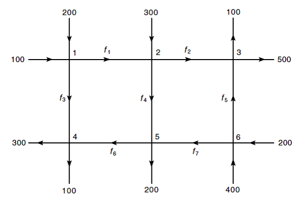 Compute
supposing that and .
Compute
supposing that and .
This example relates to the famous Google page rank algorithm.  Suppose we have a very simple internet with only four webpages
as depicted above with arrows indicating that a webpage links to another.We wish to study traffic in this network in the sense that we let a random
websurfer jump from a given webpage to another by selecting a link randomly.If you look at the network without the punctured red arrow, it is almost clear
the a random websurfer will spend % of the time uniformly in each of the
four nodes.However, if we introduce the puntured red arrow, then the percentages in
each node are given by the linear equations above. Here it turns out that
website only gets around % of the time (the other websites get double this time each).
Suppose we have a very simple internet with only four webpages
as depicted above with arrows indicating that a webpage links to another.We wish to study traffic in this network in the sense that we let a random
websurfer jump from a given webpage to another by selecting a link randomly.If you look at the network without the punctured red arrow, it is almost clear
the a random websurfer will spend % of the time uniformly in each of the
four nodes.However, if we introduce the puntured red arrow, then the percentages in
each node are given by the linear equations above. Here it turns out that
website only gets around % of the time (the other websites get double this time each).
Mentimeter
You may try out the python code below to simulate a random tour
of the small internet in Example 2.13.The list (or matrix)
A = [[0,1,0,0], [0,0,0,1], [1,1,0,0], [0,0,1,0]]
simulate(0, 1000)
2.4 Polynomials
Before going further into examples of linear equations we need to introduce (non-linear) functions called polynomials. A polynomial of degree is a function of the form where are real numbers and . We call the coefficients of . The degree of the polynomial is denoted . As an example, is a polynomial of degree with In addition to the polynomials defined in (2.6) with , we also view the function as a polynomial, called the zero polynomial. The zero polynomial does notAll its coefficients are zero! have a degree.The set of all polynomials is denoted , so that for example it makes sense to write It is probably the most natural functions from to you can come up with. If you look at (2.6), you will see that the output is formed by using addition and multiplication (by and selected real numbers).You can compute with polynomials treating the variable as a number. For example, In general a polynomial of degree times a polynomial of degree is a polynomial of degree .In the sage window below we encounter for the first time the sympy library. The input format and commands for handling polynomials should be clear from the context.You have already seen polynomials of degree one. They have the form where and are real numbers and . Similarly polynomials of degree two are called quadratic polynomials. They look like where and are real numbers and . To get a feeling for the behavior of polynomials you should experiment in the sage window below. Try varying the degree and the coefficients of the polynomial in the plot. Also adjust the plot interval for the right view.
Suppose that
To compute it seems that you need multiplications
( and ) and additions.
Can you compute with only multiplications and additions?Try to generalize to the computation of , where is a polynomial
of degree (you should only need multiplications and additions here).
2.4.1 Polynomial division
Division is sometimes referred to as long division when focusing on the method for division. Let us look at the situation for integers first.The remainder of divided by is , since Here the remainder is strictly less than the divisor .For polynomials we have a similar situation, where the degree is taken into account. For example, the remainder of divided by is , since Here the degree of the remainder is strictly less than the degree of the divisor .The Python library sympy contains a wealth of functions for symbolic mathematics. In the window below, it is shown how the polynomial division (2.7) is computed using the Polynomial Manipulaton section of the sympy documentation.The (division) algorithm for carrying out (long) division of polynomials is explained by an example in the video below.
Watch the five minute video above and
carry out (do not use a computer) the polynomial division alluded to in (2.7).
The general result about division of polynomials is given below.
Let be a non-zero polynomial. Then
for every polynomial , there exists
polynomials , such that
where or .
We will prove this using induction on . Suppose that
In general if , then
satisfies the assumptions for the identity in (2.8) with
and .If , then is a polynomial of
degree . So by induction we may find polynomials and , such that
Therefore
giving the desired result with and .
2.4.2 Roots of polynomials
A real number is called a root of the polynomial if . This is a very fundamental definition. It is mirrored beautifully in the following result.
A real number is a root of the polynomial if and only if
for some polynomial .
By Theorem 2.18, we may write
where or is a non-zero polynomial of degree zero i.e., a non-zero
constant. Now the result follows, since
using (2.9).
Is there an easy way of deciding if a polynomial of degree one divides
a polynomial without performing the (long) division of by
. Here divides means that for some polynomial .
A quadratic polynomial
has at most two roots given
by the formula (one root for and one for in below)
if its discriminant is .
Deriving the formula (2.10) comes from a classical algebraic trick called completing the square. Looking
at the quadratic equation , what bothers us is the term . If we could solve the equation rewriting to
and then taking square roots. The first step in this direction is rewriting
the equation
to
We would like to add a number to both sides of (2.11) so that the left hand side comes to look like
This is what is called completing the square.Comparing the left hand side of (2.11) with the right hand side of (2.12), we find that
works.
Therefore (2.11) implies
This identity can be rewritten into the formula (2.10) for solving the
quadratic equation.
For polynomials of degree three (cubic
polynomials) there is a formula, but these days nobody remembers it. Also for polynomials of
degree four (quartic polynomials) there is a formula. But for polynomials of degree five (quintic polynomials) and up, one can prove
that a formula cannot exist!An exceedingly important result is quoted and proved below: the degree of a polynomial is
an upper bound for its number of roots.
A non-zero polynomial of degree can have at most roots.
We will prove this by induction starting with . Here
for and
Therefore has precisely one root. Suppose now that we have proved that
polynomials of degree has at most roots. Assume that
is a polynomial of degree . If has no roots,
we are done with the proof. Suppose that i.e.,
is a root in . Then
by Proposition 2.19. Here has to be a polynomial of degree and
therefore by induction, has at most roots. However, if ,
then either or . We have proved that
cannot have more than roots.
Theorem 2.21 has a few interesting consequences. First it implies that two
identical polynomials i.e., for every must have
the same coefficients.Secondly if two polynomials and of degree satisfy
for distinct points , then
.
In Remark 2.22 it is stated that if two polynomials and of degree satisfy
for distinct points , then
. How does this follow from Theorem 2.21?
It might happen that a polynomial of degree has precisely roots, but it could have less or
even no roots: the polynomials
have no roots, whereas for example
is a quadratic polynomial with only one root. However polynomials of degree always have at
least one root.
A polynomial of odd degree always has a root.
Compute (without using a computer!) the roots of the quartic
Give an example of a polynomial of degree with precisely one root.
Suppose that are two roots of the quadratic polynomial
How can and be computed in terms of and ?
Show concretely how this can be applied to the polynomial
: if you know that how can you easily
find the other root?
Show that and use this.
2.5 Applications to polynomials
A line in the plane is given by its equation , where is the slope and is the intersection with the -axis. Two lines in the plane are either parallel or intersect in a single point.
The two lines and have a single point
of intersection. Compute this point.Give an example of two parallel lines and their equations.
Through two (distinct) points and with passes a unique line 

Notice in (2.15) that
where (for example) is a polynomial of degree two satisfying
What about and with respect to and ?
Compute the polynomial you get when you apply (2.15) to and
. How do you explain this result in terms of the
points and plotted in plane?
The natural generalization is that there exists a unique polynomial of degree passing through points
with distinct -values.The rather miraculous trick above in (2.15) is called Lagrange interpolation and can be generalized to polynomials of arbitrary degree.
Below is an example of five points defining a unique polynomial of degree four.
2.5.1 The magic of Lagrange polynomials
Let us explain with a simple numerical example what happens in (2.15). Suppose we wish to find a polynomial through the
points
More precisely we wish to find numbers and , such that
This is a system of three linear equations which in this case has a unique solution in
and .We may, however, attack this problem in another way. Suppose that and
are polynomials of degree at most two, such thatThen
really is the polynomial we wish to find.
The insight is that these and can be explicitly written down as
Compute so that
where
You can do this either by Lagrange interpolation or by solving linear equations. Which one
do you prefer?
Can you predict the next number in the sequence starting with
This question was posedThanks to Tobias Bendsen Poulsen for notifying me about this. by the tutors in a class session for new computer science students. Let us put the sequence (2.17) inside a table likewhere is the secret function responsible for the sequence. We would like to compute . Assuming that the is a polynomial function, we may simply compute the unique polynomial of degree through the points
We know how to do this either by solving linear equations or computing with Lagrange polynomials. It turns out that Sage has built in functions helping us here.Press the button to see what next number is in the sequence (computed using the secret polynomial). See also the
description of Neville's algorithm in Wikipedia for an easier approach to
computing .
2.6 Shamir secret sharing
Lagrange interpolation is used in cryptography in Shamir's secret sharing. Secret sharing is important in many practical situations. Here is an example quoted from Wikipedia:A company needs to secure their vault's passcode. They could encrypt it, but what if the beholder of the secret key is unavailable or turns rogue?One needs to distribute the secret. This is where SSS comes in. It can be used to encrypt the vault's passcode and generate a certain number of shares, where a certain number of shares can be allocated to each executive within the company. Now, only if they pool their shares can they unlock the vault. The threshold can be appropriately set for the number of executives, so the vault is always able to be accessed by the authorized individuals. Should a share or two fall into the wrong hands, they couldn't open the passcode unless the other executives cooperated.The mathematics that takes care of this is surprisingly simple. Suppose the secret is the number . Then we construct the polynomial for some other numbers . We know that this polynomial is uniquely given by its values in distinct numbers (see Remark 2.22). So if there are trusted people we could distribute the shares to them. Here we suppose that . In this setting, if there are less than of the people present they cannot open the vault. If or more people are present they can reconstruct the polynomial in (2.18), find the secret code and open the vault.
You are in a study group consisting of four people. The
professor has decided that you submit your project using a
secret code that is distributed to the group members with Shamir
secret sharing. At least three group members need to agree on
submission.On the day of the deadline three group members with shares
are present. What is the secret code they may use to submit their
project?
2.7 Fitting data
Given a data set one would often like to find a model (i.e. some function) that describes the data well. With Lagrange interpolation we can find a polynomial fitting the sample data perfectly, i.e. satisfying for . Is an optimal model? For the given data set it seems so, but we have been a bit imprecise in formulating the goal of a model.Actually, we are not very interested in modeling the data at hand with extreme precision. What we want is a model that fits new data well. Let us look at a concrete example.Consider the data set The data points , , were generated as where is a quadratic polynomial and is a random number to simulate noise. The polynomial is the best possible model for unknown data as there will always by noise that can not be modeled. In real life is what needs to be modeled based on the available data.In the figure below is a fit with a degree and degree polynomial respectively. As we see, the degree polynomial is pretty close to the target compared to the degree 10 polynomial that nevertheless fits the data perfectly. Generally a simple model is preferred over a complex, as the latter will have a tendency to fit noise. This phenomenon is called overfitting and is an extremely important topic.An interactive version of this illustration with a little more bells and whistles can be found here.