8 The Hessian

In Chapter 6 we exploited the second derivative $f''(x)$ of a one variable real function $f:(a, b) \rightarrow \RR$ to analyze convexity along with local minima and maxima.

In this chapter we introduce an analogue of the second derivative for real functions $f:\RR^d\rightarrow \RR$ of several variables. This will be a $d\times d$ matrix. The important notion of a matrix being positive (semi-) definite introduced in Section 3.7 will now make its appearance.

8.1 Introduction

In Section 6.4 the Taylor expansion for a one variable differentiable function $f:\RR\rightarrow \RR$ centered at $x_0$ with step size $h = x - x_0$ was introduced as

$f(x_0 + h) = f(x_0) + f'(x_0) h + \frac{1}{2!} f''(x_0) h^2 + \cdots \tag{8.1}$

Recall that the second derivative $f''(x_0)$ contains a wealth of information about the function. Especially if $f'(x_0) = 0$ , then we might glean from $f''(x_0)$ if $x_0$ is a local maximum or minimum or none of these (see Theorem 6.50 and review Exercise 6.53 ).

We also saw — remember the zigzag path across the narrow valley in Section 7.5.1 — that plain gradient descent can be painfully slow. Taking the second derivative into account gives a more detailed picture of the function and, as in Newton's method below, much faster algorithms.

8.2 Several variables

Our main character is a differentiable function $F:\RR^d\rightarrow \RR$ in several variables. We already know that

$F(v_0 + h) = F(v_0) + \nabla F(v_0) h + \epsilon(h) \abs{h},$ where $v_0$ and $h$ are vectors in $\RR^d$ (as opposed to the good old numbers in (8.1) ). Take a look back at Definition 7.3 for the general definition of differentiability.

We wish to have an analogue of the Taylor expansion in (8.1) for such a function of several variables. To this end we introduce the function $g:\RR\rightarrow \RR$ given by

$g(t) = F(v_0 + t h). \tag{8.2}$ Notice that

$g(t) = (F\circ A)(t),$ where $A: \RR\rightarrow \RR^d$ is the function given by $A(t) = v_0 + t h$ . In particular we get

$g'(t) = F'(v_0 + t h) h = \nabla F(v_0 + t h) h \tag{8.3}$ by using the chain rule (see Theorem 7.23 ).

Explain how the chain rule is applied to get (8.3) .

The derivative $g'(t)$ is also composed of several functions and again we may compute $g''(t)$ by using the chain rule:

$\begin{aligned} g''(t) &= (C\circ B \circ A)'(t)\\ &= (C\circ B)'(A(t)) A'(t) \\ &= C'(B(A(t))) B'(A(t)) A'(t), \end{aligned}$ where $B: \RR^d\rightarrow \RR^d$ is defined by

$B(v) = \nabla F(v)^\top$ and $C:\RR^d \rightarrow \RR$ by

$C(v) = v^\top h.$

The Hessian matrix of $F$ at the point $v\in \RR^d$ is defined by

$\nabla^2 F(v) := \begin{pmatrix} \dfrac{ \partial^2 F}{ \partial x_1 \partial x_1}(v) & \cdots & \dfrac{ \partial^2 F}{ \partial x_1 \partial x_d}(v) \\ \vdots & \ddots & \vdots \\ \dfrac{ \partial^2 F}{ \partial x_d \partial x_1}(v) & \cdots & \dfrac{\partial^2 F}{ \partial x_d\partial x_d}(v) \end{pmatrix} .$

A very important observation is that $\nabla^2 F(v)$ above is a symmetric matrix if $F$ satisfies the condition in the last part of Theorem 7.11 .

Suppose that $f: \RR^2\rightarrow \RR$ is given by

$f(x, y) = \sin(x y) + x^2 y^2 + y.$ Then the gradient

$\nabla f = \left(\frac{\partial f}{\partial x}, \frac{\partial f}{\partial y} \right)$ and the Hessian

$\nabla^2 f = \begin{pmatrix} \dfrac{\partial^2 f}{\partial x^2} & \dfrac{\partial^2 f}{\partial x \partial y} \\ \\ \dfrac{\partial^2 f}{\partial y \partial x} & \dfrac{\partial^2 f}{\partial y^2} \end{pmatrix}$ of $f$ are computed in the python cell below.

Live Python

See the calculus tutorial in the sympy documentation for more.

Verify (just this once) by hand the computations done by sympy in Example 8.3 .

Also, experiment with a few other functions in the python cell and compute their Hessians.

By applying Proposition 7.9 it is not too hard to see that the Hessian matrix fits nicely into the framework above, since

$B'(v) = \nabla^2 F(v). \tag{8.4}$

The full application of the chain rule then gives

$g''(t) = h^\top \nabla^2 F(v_0 + t h) h. \tag{8.5}$

Give a detailed explanation as to why (8.4) holds.

8.3 Newton's method for finding critical points

We may use Newton's method for computing critical points for a function $F:\RR^d\rightarrow \RR$ of several variables. Recall that a critical point is a point $v_0\in \RR^d$ with $\nabla F(v_0) = 0$ . By (7.8) and (8.4) the computation in Newton's method becomes

$v_1 = v_0 - \left(\nabla^2 F(v_0)\right)^{-1} \nabla F(v_0). \tag{8.6}$ In practice the (inverse) Hessian appearing in (8.6) is often a heavy computational burden. This leads to the socalled quasi-Newton methods, where the inverse Hessian in (8.6) is replaced by other matrices.

Let us watch (8.6) in action on the function from Exercise 7.21 ,

$f(x, y) = x^3 + x y + y^3,$ with gradient and Hessian

$\nabla f(x, y) = \begin{pmatrix} 3 x^2 + y\\ 3 y^2 + x \end{pmatrix} \qquad\text{and}\qquad \nabla^2 f(x, y) = \begin{pmatrix} 6 x & 1\\ 1 & 6 y \end{pmatrix}.$ This function offers a rare luxury: the equation $\nabla f(x, y) = (0, 0)$ can be solved by hand. The first coordinate gives $y = -3 x^2$ , and substituting this into the second,

$3 \left(-3 x^2\right)^2 + x = x \left(27 x^3 + 1\right) = 0,$ so $x = 0$ or $x = -\frac{1}{3}$ . The two critical points are

$(0, 0)\qquad\text{and}\qquad \left(-\tfrac{1}{3}, -\tfrac{1}{3}\right).$ Since we know the answers in advance, we can concentrate on how Newton's method finds them. The cell below starts at v0 and prints the point and the length of the gradient after every step of (8.6) .

Live Python

Two things in the output are worth savoring. First, the speed. Starting from $(1, 1)$ the iteration converges to $(0, 0)$ , and the lengths of the gradients fall like

$10^{-2},\quad 10^{-3},\quad 10^{-5},\quad 10^{-9},\quad 10^{-17}.$ The exponent roughly doubles in every step, so the number of correct digits doubles too. This quadratic convergence is the trademark of Newton's method — compare with the $2000$ small steps gradient ascent needed in Example 7.33 .

Second, the destination depends on the start. From $(-1, -1)$ the very same iteration converges to the other critical point $(-\frac{1}{3}, -\frac{1}{3})$ . Newton's method solves $\nabla f(x, y) = (0, 0)$ and nothing else; it has no opinion on whether the point it finds is a local minimum, a local maximum or neither. So which of the three did we just find? The answer needs the main character of this chapter, the Hessian: see Example 8.14 and Exercise 8.18 .

Run the cell in Example 8.6 with the initial point v0 = [1/6, 1/6]. What goes wrong?

Show that $\nabla^2 f(x, y)$ is invertible if and only if $36 x y \neq 1$ , so the failing initial points lie exactly on a hyperbola in the plane. If you nudge the initial point to v0 = [1/6 + 0.001, 1/6], which critical point does Newton's method find?

8.4 The Hessian and critical points

Now we are in a position to state at least the first terms in the Taylor expansion for a differentiable function $F:\RR^d\rightarrow \RR$ . The angle of the proof is to reduce to the one-dimensional case through the function $g(t)$ defined in (8.2) . Here one may prove that

$g(t) = g(0) + g'(0) t + \frac{1}{2} g''(0) t^2 + \epsilon(t)t^2, \tag{8.7}$ where $\epsilon(0) = 0$ with $\epsilon$ continuous at $0$ , much like in the definition of differentiability except that we also include the second derivative.

Now (8.7) translates into

$F(v_0 + t h) = F(v_0) + \left(\nabla F(v_0) h \right) t + \frac{1}{2} \left( h^\top \nabla^2 F(v_0) h \right) t^2 + \epsilon(t) t^2 \tag{8.8}$ by using (8.3) and (8.5) .

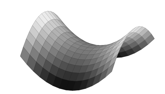
A critical point $v_0$ is called a saddle point for $F$ if there exists two vectors $u, v\in \RR^d$ , such that

$\begin{aligned} &t=0\quad \text{is a local minimum for the function}\quad F(v_0 + t u)\\ &t=0\quad \text{is a local maximum for the function}\quad F(v_0 + t v) \end{aligned}$ as illustrated in the graphics below.

Now go back and recall the definition of positive definite matrices in Section 3.7 . We call a symmetric $A$ matrix negative definite if $-A$ is positive definite. One more concept (related to the definition of saddle point above):

A symmetric $d\times d$ matrix $A$ is called indefinite if there exists $u, v\in \RR^d$ with

$\begin{aligned} u^\top A u &>0\quad\text{and}\\ v^\top A v &<0. \end{aligned}$

So an indefinite matrix is mixed up in the sense that it is neither positive definite, nor negative definite.

$\begin{aligned} \begin{pmatrix} 2 & 0 \\ 0 & 3 \end{pmatrix}\qquad &\text{is positive definite}\\ \begin{pmatrix} -2 & 0 \\ 0 & -3 \end{pmatrix}\qquad &\text{is negative definite}\\ \begin{pmatrix} 2 & 0 \\ 0 & -3 \end{pmatrix}\qquad &\text{is indefinite}\\ \begin{pmatrix} 2 & 0 \\ 0 & 0 \end{pmatrix}\qquad &\text{is neither positive definite, negative definite, nor indefinite}\\ \end{aligned}$

We have the following addition to Proposition 3.43 (with a similar proof).

Let $A$ be a symmetric $d\times d$ matrix and $B$ an invertible $d\times d$ matrix. Then $A$ is indefinite (positive definite, negative definite) if and only if

$B^\top A B$ is indefinite (positive definite, negative definite).

From (8.8) one can prove the following nice criterion, which may be viewed as a several variable generalization of Theorem 6.50 .

Let $v_0$ be a critical point for $F:\RR^d\rightarrow \RR$ . Then

$v_0$ is a local minimum if $\nabla^2 F(v_0)$ is positive definite.
$v_0$ is a local maximum if $\nabla^2 F(v_0)$ is negative definite.
$v_0$ is a saddle point if $\nabla^2 F(v_0)$ is indefinite.

Let $v_0$ be a critical point for $F:\RR^d\rightarrow \RR$ . Which of the following statements are true?

If $v_0$ is a local minimum, then $\nabla^2 F(v_0)$ is positive definite.

If $\nabla^2 F(v_0)$ is indefinite, then $v_0$ is a saddle point.

Every symmetric matrix is positive definite, negative definite or indefinite.

If $\nabla^2 F(v_0)$ is positive definite, then $v_0$ is a local minimum.

Consider, with our new technology in Theorem 8.12 , Exercise 7.21 once again. Here we analyzed the point $v_0 = (0, 0)$ for the function

$f(x, y) = x^3 + x y + y^3$ and showed (by a trick) that $v_0$ is neither a local maximum nor a local minimum for $f$ . The Hessian matrix for $f(x, y)$ at $v_0$ is

$H = \begin{pmatrix} 0 & 1 \\ 1 & 0 \end{pmatrix}.$

Now Theorem 8.12 (ⅲ) shows that $v_0$ is a saddle point, since

$\begin{pmatrix} x & y \end{pmatrix} H \begin{pmatrix} x \\ y \end{pmatrix} = 2 x y$ and

$\begin{aligned} u^\top H u &> 0\qquad\text{for } u = \begin{pmatrix} 1 \\ 1 \end{pmatrix}\\ v^\top H v &< 0\qquad\text{for } v = \begin{pmatrix} 1 \\ -1 \end{pmatrix}. \end{aligned}$

Live Python

Try plotting the graph for different values of a ¹ a=4 shows the saddle point clearly. in the python cell in Example 8.14 . What do you observe for the point $v_0$ with respect to the function? Does a have to be a number? Could it be an expression in the variables x and y like a = -10*np.cos(x)*np.sin(y)?

Check the computation of the Hessian matrix $H$ in Example 8.14 by showing that the Hessian matrix for $f$ at the point $(x, y)$ is

$\begin{pmatrix} 6 x & 1\\ 1 & 6 y \end{pmatrix}.$

What about $u$ and $v$ in Example 8.14 ? How do they relate to the hint given in Exercise 7.21 ?

Newton's method in Example 8.6 also found the critical point $\left(-\frac{1}{3}, -\frac{1}{3}\right)$ for $f(x, y) = x^3 + x y + y^3$ . Compute the Hessian of $f$ at this point and use Theorem 8.12 to decide whether it is a local minimum, a local maximum or a saddle point.

Give an example of a function $F:\RR^2\rightarrow \RR$ having a local minimum at $x_0$ , where $\nabla^2 F(x_0)$ is not positive definite.

The point $\left(0, \frac{\sqrt{3}}{3}\right)$ is a critical point for
$f(x, y) = x^3 + y^3 - y.$ What does Theorem 8.12 say about this point?
The point $\left(\frac{1}{3}, \frac{1}{3}\right)$ is a critical point for
$f(x, y) = -x^3 -x^2 + x - y^3 + 2 y^2 - y.$ What does Theorem 8.12 say about this point?
The point $(0, 1)$ is a critical point for
$f(x, y) = x^3 - x^2 + y^3 - y^2 - y.$ What does Theorem 8.12 say about this point?

Consider the function

$f(x, y) = x^4 y^2 + x^2 y^4 - 3 x^2 y^2.$ Compute its critical points and decide on their types according to Theorem 8.12 . Try to convince yourself that

$f(x, y) \geq -1$ for every $x, y\in \RR$ .

Live Python

Look at the minimization problem

$\min f(x, y)$ subject to

$(x, y)\in C = \{(x, y) \mid -M \leq x \leq M, \,\, -M \leq y \leq M\},$ where $M$ is a big number.

Give an example of a function $f:\RR\rightarrow \RR$ that has a local maximum, but where there exists $x\in \RR$ with $f(x) > M$ for any given (large) number $M$ .

8.5 Differentiable convex functions of several variables

Below is the generalization of Theorem 6.61 to several variables. You have already seen this in Exercise 6.62 , right?

Let $f: U\rightarrow \RR$ be a differentiable function, where $U\subseteq \RR^d$ is an open convex subset. Then $f$ is convex if and only if

$f(x) \geq f(x_0) + \nabla f(x_0) (x-x_0) \tag{8.9}$ for every $x, x_0\in U$ .

Proof

Suppose that (8.9) holds and let $x_t = (1-t)x_0 + t x$ with $0 \leq t \leq 1$ , where $x_0, x\in U$ . To prove that $f$ is convex we must verify the inequality

$f(x_t) \leq (1-t) f(x_0) + t f(x). \tag{8.10}$ Let $\xi = \nabla f(x_t)$ . Then

$\begin{aligned} f(x) &\geq f(x_t) + \xi (1-t) (x-x_0)\\ f(x_0) &\geq f(x_t) - \xi t (x-x_0) \end{aligned}$ by (8.9) . If you multiply the first inequality by $t$ , the second by $1-t$ and then add the two, you get (8.10) .

Suppose on the other hand that $f$ is a convex function. Let $x_0, x\in U$ . Since $U$ is an open subset, it follows that $(1-t)x_0 + t x\in U$ for $t\in I=(-\delta, 1 + \delta)$ , where $\delta>0$ is sufficiently small. Now define the function $g:I\rightarrow \RR$ by

$g(t) = f((1-t) x_0 + t x) = f(x_0 + t (x-x_0)).$ Being the composition of two differentiable functions, $g$ is differentiable. Suppose that $0\leq \alpha \leq 1$ and $t_1, t_2\in I$ . Then

$\begin{aligned} g((1- \alpha) t_1 + \alpha t_2) &= f(x_0 + ((1-\alpha) t_1 + \alpha t_2)(x-x_0)) \\ &=f((1-\alpha)(x_0 + t_1(x-x_0)) + \alpha (x_0+t_2(x-x_0))) \\ &\leq(1-\alpha) f(x_0 + t_1 (x-x_0)) + \alpha f(x_0 + t_2(x-x_0)) \\ &=(1-\alpha) g(t_1) + \alpha g(t_2) \end{aligned}$ showing that $g$ is a convex function. By Theorem 6.61 ,

$g(1) \geq g(0) + g'(0),$ which translates into

$f(x) \geq f(x_0) + \nabla f(x_0) (x-x_0)$ by using the chain rule in computing $g'(0)$ .

Prove that a bounded convex differentiable function $f:\RR^d\rightarrow \RR$ is constant.

The following is the generalization of Corollary 6.55 .

Let $f: U\rightarrow \RR$ be a differentiable function with continuous second order partial derivatives, where $U\subseteq \RR^d$ is a convex open subset. Then $f$ is convex if and only if the Hessian $\Hess{f}(x)$ is positive semidefinite for every $x\in U$ . If $\Hess{f}(x)$ is positive definite for every $x\in U$ , then $f$ is strictly convex.

Proof

We have done all the work for a convenient reduction to the one variable case. Suppose that $f$ is convex. Then the same reasoning as in the proof of Theorem 8.23 shows that

$g(t) = f(x + t v)$ is a convex function for every $x\in U$ and every $v\in \RR^d$ from an open interval $(-\delta, \delta)$ to $\RR$ for suitable $\delta>0$ . Therefore $g''(0) = v^\top \Hess{f}(x) v \geq 0$ by Theorem 6.54 . This proves that the matrix $\Hess{f}(x)$ is positive semidefinite for every $x\in U$ . Suppose on the other hand that $\Hess{f}(x)$ is positive semidefinite for every $x\in U$ . Then Theorem 6.54 shows that $g(t) = f(x + t(y-x))$ is a convex function from $(-\delta, 1+\delta)$ to $\RR$ for $\delta>0$ small and $x, y\in U$ , since

$g''(\alpha) = (y-x)^\top \Hess{f}(x + \alpha(y-x)) (y-x) \geq 0$ for $0\leq \alpha \leq 1$ . Therefore $f$ is a convex function, since

$\begin{aligned} f((1-t) x + t y) = &g((1-t)\cdot 0 + t\cdot 1) \\ &\leq(1-t) g(0) + t g(1) = (1-t) f(x) + t f(y). \end{aligned}$ The same argument (using the last part of Theorem 6.54 on strict convexity), shows that $g$ is strictly convex if $\Hess{f}(x)$ is positive definite. It follows that $f$ is strictly convex if $\Hess{f}(x)$ is positive definite for every $x\in U$ .

Prove that

$f(x, y) = x^2 + y^2$ is a strictly convex function from $\RR^2$ to $\RR$ . Also, prove that

$\{(x, y)\in \RR^2 \mid x^2 + y^2 \leq 1\}$ is a convex subset of $\RR^2$ .

Is $f(x, y) = \cos(x) + \sin(y)$ strictly convex on some non-empty open convex subset of the plane?

Show that $f:\RR^2 \rightarrow \RR$ given by

$f(x, y) = \log(e^x + e^y)$ is a convex function. Is $f$ strictly convex?

Let $f:\RR^2\rightarrow \RR$ be given by

$f(x, y) = a x^2 + b y^2 + c x y,$ where $a, b, c\in \RR$ .

Show that $f$ is a strictly convex function if and only if $a > 0$ and $4 a b - c^2 > 0$ .

This is a hint for the only if part. If $H$ is the Hessian for $f$ , then
$f(v) = \frac{1}{2} v^\top H v,$ where $v = (x, y)^\top$ - this is seen by a matrix multiplication computation. We know that $H$ is positive semidefinite. If $H$ was not positive definite, there would exist $v\neq 0$ with $f(v) = 0$ . Now use $f(t v) = t^2 f(v)$ to complete the proof that $H$ is positive definite by looking at $f((1-t)\cdot 0 + t\cdot v)$ .
Suppose now that $a > 0$ and $4 a b - c^2>0$ . Show that $g(x, y) = f(x, y) + x + y$ has a unique global minimum and give a formula for this minimum in terms of $a, b$ and $c$ .

8.6 How to decide the definiteness of a matrix

In this section we will outline a straightforward method for deciding if a matrix is positive definite, positive semidefinite, negative definite or indefinite.

Before proceeding it is a must that you do the following exercise.

Show that a diagonal matrix

$\begin{pmatrix} \lambda_1 & 0 & \dots & 0\\ 0 &\lambda_2 & \dots &0\\ \vdots & \vdots & \ddots & \vdots\\ 0 & 0 &\dots & \lambda_n \end{pmatrix}$ is positive definite if and only if $\lambda_1 > 0, \dots, \lambda_n > 0$ , positive semidefinite if and only if $\lambda_1 \geq 0, \dots, \lambda_n \geq 0$ and indefinite if and only if there exists $i\neq j$ with $\lambda_i > 0$ and $\lambda_j < 0$ .

The crucial ingredient is the following result.

Let $A$ be a real symmetric $n\times n$ matrix. Then there exists an invertible matrix $B$ , such that $B^\top A B$ is a diagonal matrix.

The proof contains an algorithm for building $B$ by different steps. We will supply examples afterwards illustrating these. An operational procedure implementing the steps is outlined in section 8.7 .

Proof

Suppose that $A=(a_{ij})$ . If $A$ has a non-zero entry in the upper left hand corner i.e., $a_{11}\neq 0$ , then

$B_1^\top A B_1 = \begin{pmatrix} a_{11} & 0 & \cdots & 0\\ 0 & c_{11} & \cdots & c_{1, n-1}\\ \vdots & \vdots & \ddots & \vdots \\ 0 & c_{n-1, 1} & \cdots & c_{n-1, n-1}, \end{pmatrix}$ where $C = (c_{ij})$ is a real symmetric matrix and $B_1$ is the invertible $n\times n$ matrix

$\begin{pmatrix} 1 & -\frac{ a_{12}}{a_{11}} & \cdots & -\frac{ a_{1n}}{a_{11}}\\ 0 & 1 & \cdots & 0\\ \vdots & \vdots & \ddots & \vdots\\ 0 & 0 & \cdots & 1 \end{pmatrix} .$ By induction on $n$ we may find an invertible matrix $(n-1)\times (n-1)$ matrix $B_2$ such that

$B_2^\top C B_2 = \begin{pmatrix} a_1 & 0 &\cdots & 0\\ 0 & a_2 & \cdots & 0\\ \vdots & \vdots & \ddots &\vdots\\ 0 & 0 & \cdots & a_{n-1} \end{pmatrix} .$

Putting

$B = B_1 \begin{pmatrix} 1 & 0\\ 0 & B_2 \end{pmatrix},$ it follows that

$B^\top A B = \begin{pmatrix} a_{11} & 0 &\cdots & 0\\ 0 & a_1 & \cdots & 0\\ \vdots & \vdots & \ddots &\vdots\\ 0 & 0 & \cdots & a_{n-1} \end{pmatrix} .$

We now treat the case of a zero entry in the upper left hand corner i.e., $a_{11}=\nobreak 0$ . Suppose first that $a_{jj} \neq 0$ for some $j > 1$ . Let $P$ denote the identity matrix with the first and $j$ -th rows interchanged. The operation $A\mapsto A P$ amounts to interchanging the first and $j$ -th columns in $A$ . Similarly $A\mapsto P^\top A$ is interchanging that first and $j$ -th rows in $A$ . The matrix $P$ is invertible and $P^\top A P$ is a symmetric matrix with $(P^\top A P)_{11} = a_{jj}\neq 0$ and we have reduced to the case of a non-zero entry in the upper left hand corner.

If $a_{ii} = 0$ for every $i = 1, \dots, n$ we may assume that $a_{1 j}\neq 0$ for some $j>1$ . Let $B$ denote the identity matrix where the entry in the first column and $j$ -th row is $1$ . The operation $A\mapsto A B$ amounts to adding the $j$ -th column to the first column in $A$ . Similarly $A\mapsto B^\top A$ is adding the $j$ -th row to the first row in $A$ . All in all we get $(B^\top A B)_{11} = 2 a_{1 j} \neq 0$ , where we have used that $a_{ii} = 0$ for $i=1, \dots, n$ . Again we have reduced to the case of a non-zero entry in the upper left hand corner.

Consider the $3\times 3$ real symmetric matrix.

$A = (a_{ij}) = \begin{pmatrix} 1 & 2 & 3\\ 2 & 8 & 4\\ 3 & 4 & 16 \end{pmatrix} .$ Here $a_{11} = 1 \neq 0$ . Therefore the fundamental step in the proof of Theorem 8.31 applies and

$\begin{pmatrix} 1 & 0 & 0 \\ -2 & 1 & 0\\ -3 & 0 & 1 \end{pmatrix} A \begin{pmatrix} 1 & -2 & -3\\ 0 & 1 & 0\\ 0 & 0 & 1 \end{pmatrix} = \begin{pmatrix} 1 & 0 & 0\\ 0 & 4 & -2\\ 0 & -2 & 7 \end{pmatrix}$ and again

$\begin{pmatrix} 1 & 0 & 0 \\ 0 & 1 & 0\\ 0 & \frac{1}{2} & 1 \end{pmatrix} \begin{pmatrix} 1 & 0 & 0\\ 0 & 4 & -2\\ 0 & -2 & 7 \end{pmatrix} \begin{pmatrix} 1 & 0 & 0\\ 0 & 1 & \frac{1}{2}\\ 0 & 0 & 1 \end{pmatrix} = \begin{pmatrix} 1 & 0 & 0\\ 0 & 4 & 0\\ 0 & 0 & 6 \end{pmatrix} .$

Summing up we get

$B = \begin{pmatrix} 1 & -2 & -3\\ 0 & 1 & 0\\ 0 & 0 & 1 \end{pmatrix} \begin{pmatrix} 1 & 0 & 0\\ 0 & 1 & \frac{1}{2}\\ 0 & 0 & 1 \end{pmatrix} = \begin{pmatrix} 1 & -2 & -4\\ 0 & 1 & \frac{1}{2}\\ 0 & 0 & 1 \end{pmatrix} .$ You are invited to check that

$B^\top A B = \begin{pmatrix} 1 & 0 & 0\\ 0 & 4 & 0\\ 0 & 0 & 6 \end{pmatrix} .$

Let

$A = \begin{pmatrix} 0 & 0 & 1 & 1\\ 0 & 0 & 2 & 3\\ 1 & 2 & 1 & 4\\ 1 & 3 & 4 & 0 \end{pmatrix}.$ Here $a_{11} = a_{22} = 0$ , but the diagonal element $a_{33}\neq 0$ . So we are in the second step of the proof of Theorem 8.31 . Using the matrix

$P = \begin{pmatrix} 0 & 0 & 1 & 0\\ 0 & 1 & 0 & 0\\ 1 & 0 & 0 & 0\\ 0 & 0 & 0 & 1 \end{pmatrix}$ we get

$P^\top A P = \begin{pmatrix} 1 & 2 & 1 & 4\\ 2 & 0 & 0 & 3\\ 1 & 0 & 0 & 1\\ 4 & 3 & 1 & 0 \end{pmatrix} .$

As argued in the proof, this corresponds to interchanging the first and third columns and then interchanging the first and third rows. In total you move the non-zero $a_{33}$ to the upper left corner in the matrix.

Consider the symmetric matrix

$A = \begin{pmatrix} 0 & 1 & 1 & 1\\ 1 & 0 & 1 & 1\\ 1 & 1 & 0 & 1\\ 1 & 1 & 1 & 0 \end{pmatrix} .$ We have zero entries in the diagonal. As in the third step in the proof of Theorem 8.31 we must find an invertible matrix $B_1$ , such that the upper left corner in $B_1^\top A B_1$ is non-zero. In the proof it is used that every diagonal element is zero: if we locate a non-zero element in the $j$ -th column in the first row, we can add the $j$ -th column to the first column and then the $j$ -th row to the first row obtaining a non-zero element in the upper left corner. For $A$ above we choose $j=2$ and the matrix $B_1$ becomes

$B_1 = \begin{pmatrix} 1 & 0 & 0 & 0\\ 1 & 1 & 0 & 0\\ 0 & 0 & 1 & 0\\ 0 & 0 & 0 & 1 \end{pmatrix}$ so that

$B_1^\top A B_1 = \begin{pmatrix} 2 & 1 & 2 & 2\\ 1 & 0 & 1 & 1\\ 2 & 1 & 0 & 1\\ 2 & 1 & 1 & 0 \end{pmatrix} .$

Let $A$ be any matrix. Show that

$A^\top A$ is positive semidefinite.

Which of the following statements about symmetric matrices $A$ are true?

A symmetric matrix with a diagonal entry equal to $0$ cannot be positive definite.

$A^\top A$ is positive semidefinite for every matrix $A$ .

Every symmetric matrix is either positive semidefinite or negative semidefinite.

A symmetric matrix with all diagonal entries positive is positive definite.

Find inequalities defining the set

$\left\{(a, b)\in \RR^2 \middle\vert \begin{pmatrix} 2 & 1 & a\\ 1 & 1 & 1 \\ a & 1 & b \end{pmatrix} \,\,\text{is positive definite} \right\}.$ Same question with positive semidefinite. Sketch and compare the two subsets of the plane $\{(a, b) \mid a, b\in \RR\}$ .

Let $f:\RR^3\rightarrow \RR$ denote the function given by

$f(x, y, z) = x^2 + y^2 + z^2 + a x y + x z + y z,$ where $a\in \RR$ . Let $H$ denote the Hessian of $f$ in a point $(x, y, z)\in \RR^3$ .

Compute $H$ .
Show that $f(v) = v^\top A v$ for $v=(x, y, z)\in \RR^3$ and $A = \frac{1}{2} H$ .
Compute a non-zero vector $v\in \RR^3$ , such that $H v = 0$ in the case, where $a=2$ . Is $H$ invertible in this case?
Show that $f$ is strictly convex if $-1 < a < 2$ .
Is $f$ strictly convex if $a=2$ ?

Hint
Consider the line segment between $0$ and a suitable vector $u\neq 0$ , where $f(u) = 0$ .

Why is the subset given by the inequalities

$\begin{aligned} x &\geq 0\\ y &\geq 0\\ x y - z^2 &\geq 0 \end{aligned}$ a convex subset of $\RR^3$ ?

8.7 A schematic procedure for transforming symmetric matrices

Suppose that $A$ is a symmetric $n\times n$ matrix. We wish to find an invertible matrix $B$ and a diagonal matrix $D$ so that

$B^\top A B = D.$ Every step in the algorithm in the proof of Theorem 8.31 involve an operation on the columns of $A$ followed by a similar operation on the rows. These steps can be carried out systematically by transforming the extended $(2 n)\times n$ matrix

$\begin{pmatrix} I_n \\ A \end{pmatrix}\qquad\qquad\text{into}\quad\quad \begin{pmatrix} B \\ D \end{pmatrix}. \tag{8.11}$ The recipe is: every column operation (on $A$ ) is carried out on the full $(2 n)\times n$ matrix, whereas every row operation is only carried out on the lower $n\times n$ matrix in (8.11) .

Here is how this plays out for the examples above.

Here is the schematic procedure applied to Example 8.32 :

$\begin{aligned} &\begin{pmatrix} 1 & 0 & 0 \\ 0 & 1 & 0\\ 0 & 0 & 1\\ 1 & 2 & 3\\ 2 & 8 & 4\\ 3 & 4 & 16 \end{pmatrix}\rightarrow \begin{pmatrix} 1 & -2 & 0 \\ 0 & 1 & 0\\ 0 & 0 & 1\\ 1 & 0 & 3\\ 2 & 4 & 4\\ 3 & -2 & 16 \end{pmatrix}\rightarrow \begin{pmatrix} 1 & -2 & 0 \\ 0 & 1 & 0\\ 0 & 0 & 1\\ 1 & 0 & 3\\ 0 & 4 & -2\\ 3 & -2 & 16 \end{pmatrix}\rightarrow &\begin{pmatrix} 1 & -2 & -3 \\ 0 & 1 & 0\\ 0 & 0 & 1\\ 1 & 0 & 0\\ 0 & 4 & -2\\ 3 & -2 & 7 \end{pmatrix}\rightarrow\\ &\\ &\begin{pmatrix} 1 & -2 & -3 \\ 0 & 1 & 0\\ 0 & 0 & 1\\ 1 & 0 & 0\\ 0 & 4 & -2\\ 0 & -2 & 7 \end{pmatrix}\rightarrow \begin{pmatrix} 1 & -2 & -4 \\ 0 & 1 & \frac{1}{2}\\ 0 & 0 & 1\\ 1 & 0 & 0\\ 0 & 4 & 0\\ 0 & -2 & 6 \end{pmatrix}\rightarrow \begin{pmatrix} 1 & -2 & -4 \\ 0 & 1 & \frac{1}{2}\\ 0 & 0 & 1\\ 1 & 0 & 0\\ 0 & 4 & 0\\ 0 & 0 & 6 \end{pmatrix}. \end{aligned}$

Here is the schematic procedure applied to Example 8.33 :

$\begin{pmatrix} 1 & 0 & 0 & 0\\ 0 & 1 & 0 & 0\\ 0 & 0 & 1 & 0\\ 0 & 0 & 0 & 1\\ 0 & 0 & 1 & 1\\ 0 & 0 & 2 & 3\\ 1 & 2 & 1 & 4\\ 1 & 3 & 4 & 0 \end{pmatrix}\rightarrow \begin{pmatrix} 0 & 0 & 1 & 0\\ 0 & 1 & 0 & 0\\ 1 & 0 & 0 & 0\\ 0 & 0 & 0 & 1\\ 1 & 0 & 0 & 1\\ 2 & 0 & 0 & 3\\ 1 & 2 & 1 & 4\\ 4 & 3 & 1 & 0 \end{pmatrix}\rightarrow \begin{pmatrix} 0 & 0 & 1 & 0\\ 0 & 1 & 0 & 0\\ 1 & 0 & 0 & 0\\ 0 & 0 & 0 & 1\\ 1 & 2 & 1 & 4\\ 2 & 0 & 0 & 3\\ 1 & 0 & 0 & 1\\ 4 & 3 & 1 & 0 \end{pmatrix}.$

Here is the schematic procedure applied to Example 8.34 :

$\begin{pmatrix} 1 & 0 & 0 & 0\\ 0 & 1 & 0 & 0\\ 0 & 0 & 1 & 0\\ 0 & 0 & 0 & 1\\ 0 & 1 & 1 & 1\\ 1 & 0 & 1 & 1\\ 1 & 1 & 0 & 1\\ 1 & 1 & 1 & 0 \end{pmatrix}\rightarrow \begin{pmatrix} 1 & 0 & 0 & 0\\ 1 & 1 & 0 & 0\\ 0 & 0 & 1 & 0\\ 0 & 0 & 0 & 1\\ 1 & 1 & 1 & 1\\ 1 & 0 & 1 & 1\\ 2 & 1 & 0 & 1\\ 2 & 1 & 1 & 0 \end{pmatrix}\rightarrow \begin{pmatrix} 1 & 0 & 0 & 0\\ 1 & 1 & 0 & 0\\ 0 & 0 & 1 & 0\\ 0 & 0 & 0 & 1\\ 2 & 1 & 2 & 2\\ 1 & 0 & 1 & 1\\ 2 & 1 & 0 & 1\\ 2 & 1 & 1 & 0 \end{pmatrix}.$

The schematic procedure is exactly the kind of mechanical recipe a computer is made for. In the cell below the computer does the exact arithmetic — you step through the algorithm with the Next button. Run the cell, then press Next~ $\blacktriangleright$ : every press performs one arrow from the chains above — a column operation on the whole extended matrix, or the matching row operation on the lower half — and highlights the entries that changed. Watch $B$ being built in the upper half while $A$ is hammered into the diagonal matrix $D$ in the lower half. Step back and forth until every move makes sense, then replace A with the matrices from Examples 8.33 and 8.34 — the stepper knows the swap and the zero-diagonal trick from the proof of Theorem 8.31 — or with a symmetric matrix of your own.

Live Python

from sympy import Matrix, eye

A = Matrix([[1, 2, 3],
            [2, 8, 4],
            [3, 4, 16]])
# also try:
# A = Matrix([[0, 0, 1, 1], [0, 0, 2, 3], [1, 2, 1, 4], [1, 3, 4, 0]])
# A = Matrix([[0, 1, 1, 1], [1, 0, 1, 1], [1, 1, 0, 1], [1, 1, 1, 0]])

n = A.rows
ext = eye(n).col_join(Matrix(A))   # extended matrix: I on top of a copy of A
steps = []

def snap(msg, changed=()):    # snapshot for the interactive stepper
    steps.append({"msg": msg,
                  "m": [[str(ext[r, c]) for c in range(n)]
                        for r in range(2*n)],
                  "ch": [list(rc) for rc in changed]})

def addpair(i, j, c):         # the two arrows of one add operation
    ext[:, j] += c*ext[:, i]
    snap(f"Add ({c}) times column {i+1} to column {j+1} -- "
         f"column operations hit the whole extended matrix.",
         [(r, j) for r in range(2*n)])
    ext[n+j, :] += c*ext[n+i, :]
    snap(f"Add ({c}) times row {i+1} to row {j+1} -- "
         f"row operations only hit the lower half.",
         [(n+j, col) for col in range(n)])

def swappair(i, j):           # the two arrows of one swap
    ext.col_swap(i, j)
    snap(f"Interchange columns {i+1} and {j+1} in the whole matrix.",
         [(r, cc) for r in range(2*n) for cc in (i, j)])
    ext.row_swap(n+i, n+j)
    snap(f"Interchange rows {i+1} and {j+1} in the lower half.",
         [(rr, cc) for rr in (n+i, n+j) for cc in range(n)])

snap("The extended matrix: the identity on top of A. "
     "Press Next to watch the schematic procedure unfold.")

for k in range(n):
    if ext[n+k, k] == 0:      # swap a nonzero diagonal entry up
        for j in range(k+1, n):
            if ext[n+j, j] != 0:
                swappair(k, j); break
    if ext[n+k, k] == 0:      # diagonal all zero: the adding trick
        for j in range(k+1, n):
            if ext[n+k, j] != 0:
                addpair(j, k, 1); break
    if ext[n+k, k] != 0:      # clear row and column k
        for j in range(k+1, n):
            if ext[n+k, j] != 0:
                addpair(k, j, -ext[n+k, j]/ext[n+k, k])

d = [ext[n+k, k] for k in range(n)]
snap(f"Done: the lower half is the diagonal matrix D, "
     f"the upper half is B, and B^T A B = D. "
     f"Read the definiteness of A off the diagonal: {d}.")

show_steps(steps, split=n)    # stepper widget provided by the page

In the button below is a complete implementation. The function diagonalize carries out the steps from the proof of Theorem 8.31 , returning the matrices $B$ and $D$ , and definiteness reads the answer off the diagonal of $D$ . Try it on the examples above and check it against the steps in the widget.

Complete implementation

Live Python

from sympy import Matrix, eye, pprint

def diagonalize(A):
    """Return (B, D) with B invertible and B.T * A * B = D diagonal.

The schematic procedure: we walk through the corners
    k = 1, ..., n; every column operation is applied to both
    B and A, the matching row operation only to A."""
    A = Matrix(A)   # a working copy; entries become exact fractions
    n = A.rows
    B = eye(n)

for k in range(n):
        if A[k, k] == 0:
            # swap a later nonzero diagonal entry into the corner
            for j in range(k + 1, n):
                if A[j, j] != 0:
                    B.col_swap(k, j)
                    A.col_swap(k, j)
                    A.row_swap(k, j)
                    break
        if A[k, k] == 0:
            # diagonal is all zero: add column (and row) j, making
            # the corner 2*A[k, j] != 0
            for j in range(k + 1, n):
                if A[k, j] != 0:
                    B[:, k] = B[:, k] + B[:, j]
                    A[:, k] = A[:, k] + A[:, j]
                    A[k, :] = A[k, :] + A[j, :]
                    break
        if A[k, k] != 0:
            # clear row and column k using the nonzero corner
            for j in range(k + 1, n):
                c = -A[k, j] / A[k, k]
                B[:, j] = B[:, j] + c * B[:, k]
                A[:, j] = A[:, j] + c * A[:, k]
                A[j, :] = A[j, :] + c * A[k, :]

return B, A

def definiteness(A):
    _, D = diagonalize(A)
    d = list(D.diagonal())
    if all(x > 0 for x in d): return "positive definite"
    if all(x < 0 for x in d): return "negative definite"
    if all(x >= 0 for x in d): return "positive semidefinite"
    if all(x <= 0 for x in d): return "negative semidefinite"
    return "indefinite"

A = Matrix([[1, 2, 3],
            [2, 8, 4],
            [3, 4, 16]])

B, D = diagonalize(A)
print("B =");  pprint(B)
print("D = B^T A B ="); pprint(D)
print("check:", B.T * A * B == D)
print("A is", definiteness(A))

The algorithm you have just seen is old. In 1759, the 23-year-old Joseph-Louis Lagrange published Recherches sur la méthode de maximis et minimis, asking precisely the question of this chapter: when is a critical point of a function of several variables a minimum? His answer amounted to repeatedly completing the square in the second order term — in modern language, the diagonal entry $a_{kk}$ is used to eliminate the mixed terms, which is exactly step one of our procedure. For this reason the method is still known as Lagrange reduction of a quadratic form. The bookkeeping with matrices came much later. The systematic treatment, including the tricks for a vanishing diagonal, was collected in Felix Gantmacher's The Theory of Matrices (1953, English translation 1959), for decades the standard reference on the subject and still in print. It is a pleasant thought that when you press Run in the cells above, your browser is carrying out, step by step, a computation Lagrange did by hand more than 250 years ago.