5 Euclidean vector spaces
5.1 Vectors in the plane
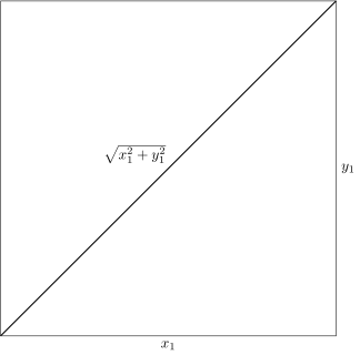
5.2 Higher dimensions
5.2.1 Dot product, norm and cosine
Suppose that
are vectors in .
-
The dot product between and
is defined by
-
Two vectors are called orthogonal if . We write
this as .
-
The norm of is defined by
-
The distance between the two vectors and is defined by
-
The cosine of the angle between and is defined by
provided that they both are non-zero.
Live Python
Your first machine learning algorithm
Live Python
Show that
where .
Use the definition in
(5.3)
to show that
for and .
Let be a nonzero vector and . Use the definition
in
(5.4)
to show that
and that
is a unit vector.
You could perhaps use Exercise
5.4
to do this. Notice also that
is the absolute value for if .
Given two vectors with , find , such
that and are orthogonal, i.e.
For , it is sketched below
that if and are orthogonal, then
and are the sides in a right triangle.
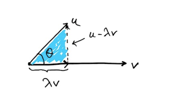 In this case, if is the angle between and , show that
Use this to show that
Finally show that
where and are two angles.
In this case, if is the angle between and , show that
Use this to show that
Finally show that
where and are two angles.
This is an equation, where is unknown!
In the last question, you could use that the vectors
are unit vectors.
Given two vectors , solve the minimization problem
First convince yourself that minimizes
if and only if it minimizes
which happens to be a quadratic polynomial in .
5.3 The unreasonable effectiveness of the dot product
5.3.1 The dist formula from high school
The infamous dist formula from high school says that the distance from the point to the line given by is Where does this magical formula come from? Consider a general line in parametrized form (see Definition 4.12 ) If , then the distance from to is given by the solution to the optimization problem This looks scary, but simply boils down to finding the top of a parabola. The solution is and the point on closest to is .Live Python
5.3.2 The perceptron algorithm
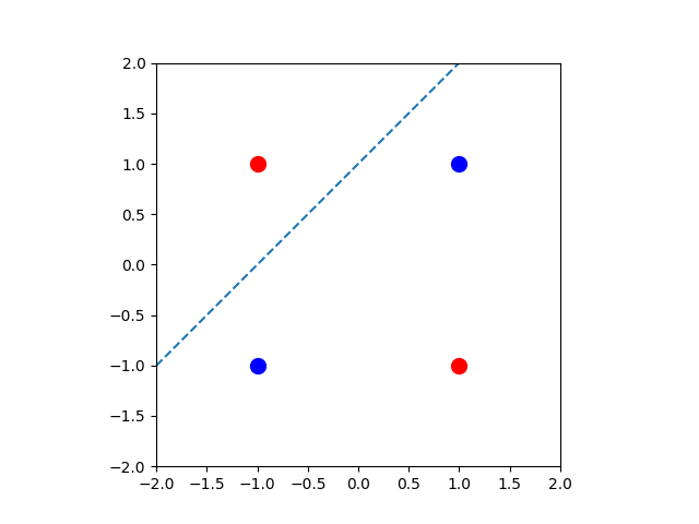
Show that it is impossible to find a line separating the red and blue points above. The red points are
and . The blue points are and .
A ridiculously simple algorithm
Given finitely many vectors , can we find
, such that
for every ?
Come up with a simple example, where this problem is unsolvable i.e., come
up with vectors , where such an does not
exist.
Hint
Try out some simple examples for and .
- Begin by putting .
- If there exists with , then replace by and repeat this step. Otherwise is the desired output vector.
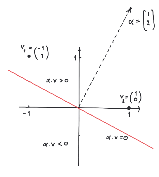
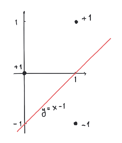
Consider the points
in , where and are labeled by and is labeled by . Then we let
Now we run the simple algorithm above Example
5.11
:
From the last vector we see that determines
a line separating the labeled points.
Live Python
Live Python
Consider the points
in , where the first point is labeled with and the rest by .
Use the perceptron algorithm to compute a separating hyperplane.
What happens when you run the perceptron algorithm on the above
points, but where the label of
is changed from to ?
5.3.3 Why does the perceptron algorithm work?
We will assume that there exists , such that for every . Therefore and if we put then for every .
Let .
After iterations of the perceptron algorithm, satisfies
where is defined in
(5.9)
.
The algorithm starts with . In the second step we update to
if . For such a we have the following
inequalities
and
If the second step of the algorithm is executed after steps, then we get for the new
that
5.4 Pythagoras and the least squares method
If and , then
This follows from
since .
Suppose we know that is orthogonal to for every . Then
for every
by Proposition
5.15
. So, in the case that
for every we have
for every proving that is an optimal solution to
(5.12)
.
Now we wish to show that is orthogonal to for every if and
only if . This is a computation involving the matrix arithmetic
introduced in Chapter
3
:
for every if and only if . But
so that .
On the other hand, if for every , then for
every : if we could find with , then
for a small number . This follows, since
which is
By picking sufficiently small,
Show that
(5.11)
has no solutions. Compute the best approximate solution to
(5.11)
using Theorem
5.16
.
The classical application of the least squares method is to find
the best line through a given set of points
in the plane .
Usually we cannot find a line matching the points precisely. This corresponds to the fact that
the system of equations
has no solutions.
Working with the least squares solution, we try to compute the best
line in the sense that
is minimized.
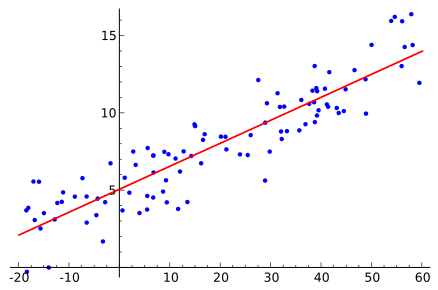
Best fit of line to random points from Wikipedia.
We might as well have asked for the best quadratic polynomial
passing through the points
in .
The same method gives us the system
of linear equations.
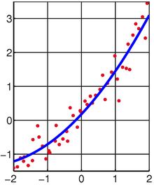
Best fit of quadratic polynomial to random points from Wikipedia.
The method generalizes naturally to finding the best polynomial of degree
through a given set of points.
Live Python
Find the best line through the points
and and the best quadratic polynomial
through the points
and .
It is important here, that you write down the relevant system
of linear equations according to Theorem
5.16
.
It is however ok to solve the equations
on a computer (or check your best fit on WolframAlpha).
Also, you can get a graphical illustration of your result in the python cell below.
Live Python
Eight students studied hours for an exam and either failed
() or passed ():
Find the best line through these eight points
(set up the normal equations from Theorem
5.16
; solving them
on a computer is fine — the cell below plots your line over the
data). It is tempting to read the line's value at as "the chance
of passing after hours of study". Compute the line's value at
and at . Why do the two numbers make that reading
absurd? Something better is needed for yes/no data — that something
is the sigmoid function, and it arrives in Chapter
7
where these eight students return.
Live Python
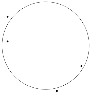
A circle with center and radius is given by the equation
-
Explain how
(5.14)
can be rewritten to the equation
where .
-
Explain how fitting a circle to the points
in the least squares context using
(5.15)
leads to the system
of linear equations.
- Compute the best circle through the points by giving the center coordinates and radius with two decimals. Use the python cell below to plot your result too see if it matches the drawing.
Live Python
5.5 The Cauchy-Schwarz inequality
For two vectors ,
If both sides are , so we may assume .
We consider the function given by
Then is a quadratic polynomial with . Therefore
its discriminant must be i.e.,
which gives the result.
Why are the two inequalities
a consequence of Theorem
5.24
?
For arbitrary two numbers ,
since
Why is
for arbitrary numbers ?
5.5.1 The triangle inequality
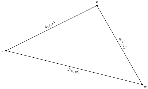
(5.27) COROLLARY (Triangle inequality).
For three vectors ,
From the Cauchy-Schwarz inequality (Theorem
5.24
) it follows that
for two vectors .
Since the right hand side of this inequality is , we have
By the definition of , we then get the desired inequality as
Apply the triangle inequality in the form
for to show that
upload or paste your solution
5.5.2 Cosine similarity in machine learning
'a', 'and', 'applicable', 'are', 'fun', 'is', 'mathematics', 'matrices', 'matrix', 'useful'Each word gets embedded into with a vector associated to its row below
Live Python
Live Python
Use the cell above to compute the cosine similarity between the two
one-word sentences "matrix" and "matrices" — and between "fun" and
"boring". Explain the outcome. Is it reasonable?
Live Python
Live Python
Live Python
5.5.3 Attention: vectors that depend on context
Keep the initial vector for "bank" fixed. Change only its context,
and watch its updated vector change.
Live Python
Experiment with the two contexts in the cell above.
- Set . Compute the weights, the gathered vector and the updated vector by hand for each context.
- Restore . Why does "today" receive so little weight? Remove it from both contexts and compare the outputs.
- Try the mixed context "river, loan, today". Predict which of the first two coordinates will be larger. What happens as grows? Explain why there is no unique nearest neighbor.
The claims made about the dial deserve proofs. Let
be the scores in
(5.17)
.
- Show that for all and that , no matter the value of and the signs of the scores.
- Suppose for all . Show that as .
For the second part, divide the numerator and the denominator of
by :
Every exponent tends to as
, since .
5.6 Special subsets of euclidean spaces
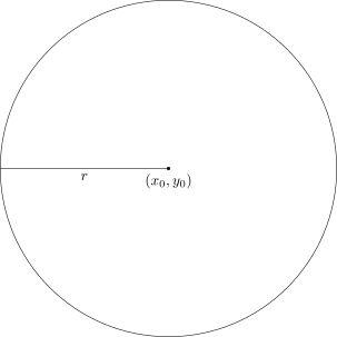
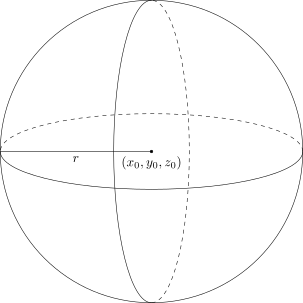
The open ball centered at with radius is defined as
5.6.1 Bounded subsets
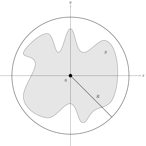
A subset is called bounded if there exists , such that
(5.34) REMARK (The logic of boundedness).
Spelled out with quantifiers, Definition
5.33
says
Read it aloud: there is one radius that works for
every point of at the same time. This is where many
stumble, because swapping the two quantifiers gives the statement
which is true for every subset whatsoever: given , choose
. The swapped statement says nothing — choosing
after seeing is cheating. In the definition must be chosen
first, and then survive all . The order of and
is everything.
For the same reason, showing that a subset is not bounded
amounts to proving the negation
i.e., no matter which radius is proposed, some point of escapes
the ball.
It does not matter whether we demand or above:
if for every , then also for every
, and is just another radius. With this in mind,
boundedness of is equivalent to each of the following two
conditions.
- There exists , such that for every . This says , which is the same as .
- There exists , such that for and every i.e., no single coordinate can run off to infinity. Here gives one direction and the other.
Chatbot Prompt
I find the definition below quite hard to understand. It is about bounded subsets. Please explain it to me patiently, give some examples and test me afterwards. ''' A subset $S \subseteq \mathbb{R}^n$ is called bounded if there exists $R\in \mathbb{R}$, such that
$$
S \subseteq B(0, R),
$$
where $B(0, R) =  \{v\in \mathbb{R}^n \mid d(0, v) < R\}$ and $d$ is the euclidean distance function. '''
Show precisely that the subset of is not bounded, whereas the subset
is.
Hint
Use the negation from Remark
5.34
: given any
proposed radius , you must point to a natural number with
(this is the archimedean property of the real numbers
from the first chapter).
Sketch why
is bounded. Now use Fourier-Motzkin elimination to show the same
without sketching.
5.6.2 Open, closed and compact subsets and boundaries and interiors of subsets
Open subsets
An open subset of is a subset consisting of points, that are interior in the following sense: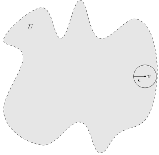
A subset is called open if for every , there exists , such that
The interval is an open subset of : for
the ball is contained
in if we choose — the wiggle
room shrinks as approaches or , but it never vanishes.
The interval is not open: the point has no
wiggle room at all, since
contains negative numbers for every .
The empty set and itself are both open. For
, every works at every point. For , the
condition is an all-statement over the empty set — true for the same
reason that was true in the quiz from
the first chapter.
Decide whether each of the subsets given below are open.
- (the -axis in )
Prove that an open ball given by is an open subset.
Suppose that . Define a suitable for and use
Corollary
5.27
to conclude that .
Show that a finite subset of is never open.
If are open subsets, then
are open subsets.
Let . Then for some , and
since is open there exists with
.
Let . For each there exists
with . Put
. Then
for every ,
so .
The proposition above concerns finitely many open subsets. Show that
and that is not an open subset of . Where does the proof
above break down for infinitely many subsets?
Closed subsets
A subset is called closed if is open.
Closed is not the opposite of open — subsets are not doors. A
subset can be both open and closed ( and ), and it
can be neither: is not open (no wiggle room at ) and not
closed (its complement has no wiggle
room at ).
If are closed subsets, then
are closed subsets.
Decide whether each of the subsets given below are closed.
Open intervals
The following subsets
are open subsets of for every .
Let us prove that is an open subset of .
If , then we let .
Suppose that . If , then and .
If , then and therefore and .
We have proved that is an open subset.
A similar proof shows that is an open subset. If , then
which is an open subset by the above and Proposition
5.45
.
Closed intervals
The following subsets
are closed subsets of for every .
Compact subsets
A subset is called compact if it is bounded and closed.
The interval is compact: bounded and closed. The interval
is bounded but not closed, and the continuous function
has no minimum on it: for every there are
smaller numbers in , and the natural candidate does not
belong to the subset. The subset is closed but not bounded, and
has no minimum on it either — this time it escapes to
.
The boundary of a subset
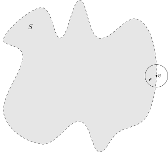
The boundary of a subset is defined as
What is the boundary of ? What about ?
The interior of a subset
The interior of a subset is defined by
Prove that the interior of any subset is
an open subset. Then show that is open if and only if
.
Let and .
First make a sketch of these two subsets in and respectively. Then
find and .
5.7 Continuous functions
The limit of a function at a point
(5.61) REMARK (The – game).
Fix a function , a point and a candidate limit
. A skeptic challenges you:
You win the round if your delivers: every input
within distance of must have within distance
of . The limit of at is if you can win every
round, no matter how small an the skeptic demands. The
smaller the skeptic's , the smaller you will typically have
to choose your .
Skeptic: I demand that the output stays within of .You: Then keep the input within of . I promise that suffices.
Let be a function, where and
, let and let . We write
and say that has limit as approaches , if
Consider
a function defined on : at both
numerator and denominator vanish and the formula breaks down. And yet
approaches a definite value as approaches , because
for every . So
and the game is easy to win: if the skeptic demands , answer
, since
for every with . Notice that the limit
exists even though does not: the limit only speaks about the
values of near .
What is
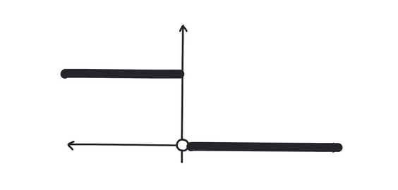
Does exist for the jump function
(5.18)
?
Hint
For the jump function: whichever candidate limit is proposed, the
skeptic demands . Every -strip around
contains inputs with output and inputs with output — can
both be within of ?
Continuity
A function , where and
, is called continuous at if
The function is called continuous if it is continuous at every
. Unfolded via Definition
5.62
, continuity
of at says
i.e., you can win the – game with .
Chatbot Prompt
I find the two definitions below (the limit of a function at a point, and continuity) challenging to understand. Please explain them to me patiently with lots of examples, including the interpretation as a game between me and a skeptic. Test me in the end. ''' Let $f: S\rightarrow T$, where $S \subseteq \mathbb{R}^m$ and $T\subseteq \mathbb{R}^d$, let $v\in \mathbb{R}^m$ and $w\in \mathbb{R}^d$. We write $\lim_{u\to v} f(u) = w$ if
$$
\forall \epsilon > 0\, \exists \delta > 0\, \forall u\in S: d(u, v) < \delta \implies d(f(u), w) < \epsilon.
$$
The function $f$ is continuous at $v\in S$ if $\lim_{u\to v} f(u) = f(v)$. '''
Live Python
Let in Definition
5.65
. We consider the two functions
where i.e., is the identity function and is a
constant function given by the real number . Both of these
functions are continuous. Let us see why.
For the function ,
(5.20)
reads
This is certainly true if we pick : you win the
game by echoing the skeptic's demand.
For the function ,
(5.20)
reads
Here can be picked arbitrarily, since is always true —
against a constant function the skeptic never stood a chance.
the prompt carries the passage above
5.7.1 An elegant way of characterizing a continuous function
Let be a function. Then is continuous if and only if
is open in for every open subset .
Let be an open subset.
Assume first that is continuous.
We wish to prove that
is open. Pick and so that
. Now use the continuity of to pick
so that
(5.20)
is satisfied i.e.,
Since ,
(5.21)
says that
showing that is an open subset.
Now suppose that is open whenever is open.
For and we put .
Since is an open subset, is open and .
So we may find so that .
But this is exactly the statement that
showing that is continuous.
If is a closed subset and
a continuous function, then the preimage
is a closed subset of .
If is closed, then is open. Therefore
is open by Proposition
5.68
. This implies that is closed.
Let us assume for now that given by is
continuous (see Exercise
5.76
). Then Proposition
5.69
shows that the subset
of is closed, since is a closed subset
of by Proposition
5.52
.
Show formally that the subset
is an open subset of .
5.7.2 Working with continuous functions
The projection functions defined in Definition
1.104
are continuous. In general a function
is continuous if and only if
is continuous for every , where and
.
Lemma
5.72
shows for example that the functions and
are continuous functions from to .
Consider the vector function given by
as an example. To prove that is continuous, Lemma
5.72
tells us that it
is enough to prove that its coordinate functions
are continuous.
Suppose that and are continuous
functions, where and . Then
the composition
is continuous.
Let be functions defined on a subset . If
and are continuous, then the functions
are continuous functions, where (the last function is
defined only if ).
This result is a consequence of the definition of continuity and Proposition
5.74
.
Show in detail that the function given by
is continuous by using Proposition
5.75
combined with
Lemma
5.72
.
Verify the claim in Remark
5.77
.
More advanced (transcendental) functions like and also turn out to be continuous.
We will return to this in the next chapter, where differentiable functions are defined.
Show from scratch (without using Remark
5.77
) that
is a continuous function , where and and
Use Proposition
5.52
and Proposition
5.69
to show that
is a closed subset of .
Hint
Does
exist? What about
Write
where is a suitable (closed) interval.
5.8 Important and special results for continuous functions
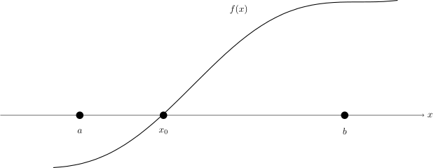
Let be a continuous function, where . If
and , then there exists with , such
that .
The idea behind Bolzano's theorem is not just theory — it is the
bisection algorithm for solving equations: cut the interval in
half, keep the half where the sign changes, repeat. Below it hunts
down a root of , i.e., the cube root of . Fifty
halvings of trap the root in an interval of length
.
Live Python
Use the methods of Example
1.83
to show that
there is no with , where .
Let
be a polynomial of odd degree, i.e. is odd and . Then has a root,
i.e. there exists , such that .
We will assume that (if not, just multiply by ). Consider written as
By choosing negative with extremely big, we have ,
since is negative and
as is positive. Notice here that the terms
are extremely small, when is extremely big.
Similarly by choosing
positive and tremendously big, we have .
By Theorem
5.81
, there exists with with
.
Let be a compact subset of and
a continuous function. Then there exists , such that
for every .
Give two examples, where Theorem
5.84
fails for if we relax
the conditions on .
One, where is open and another one where is not bounded.