6 Convex functions

In this chapter we will dive deeper into convex functions. The main focus will be on (differentiable) convex functions defined on intervals (convex subsets) of the real numbers i.e. (differentiable) convex functions in just one variable. Along the way, differentiability is formally introduced. I will assume that you are familiar with differentiation in an operational manner.

6.1 Strictly convex functions

Below we strengthen Definition 4.26 of a convex function.

Let $C \subseteq \RR^d$ be a convex subset. A strictly convex function is a convex function $f: C\rightarrow \RR$ , such that

$f((1 - t) u + t v) < (1-t) f(u) + t f(v) \tag{6.1}$ for every number $t$ with $0< t < 1$ and every $u, v\in C$ with $u\neq v$ .

The strict inequality in (6.1) collapses to an equality if $u=v, t = 0$ or $t=1$ . For example, if $u=v$ , then the left hand side of (6.1) is $f((1-t) u + t u) = f(u)$ and the right hand side is $(1-t)f(u) + t f(u) = f(u)$ .

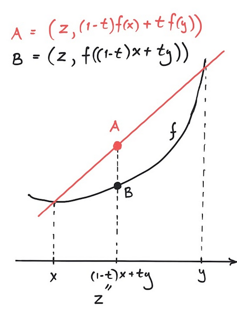
Definition 6.1 is illustrated below for a function $f:\RR\rightarrow \RR$ . Here both $u=x$ and $v=y$ are real numbers (that is, $d=1$ in $\RR^d$ in Definition 6.1 ). The (red) line segment between $(x, f(x))$ and $(y, f(y))$ lies strictly ( $<$ ) above the (black) graph of $f$ :

Chatbot Prompt

Please explain patiently the definition below to me. It seems that it is also valid for functions defined on vectors in the plane ($d=2$). Give concrete examples of this. Test me with a few questions in the end. ''' Let $C \subseteq \mathbb{R}^d$ be a convex subset. A \emph{strictly convex function} is a convex function $f: C\rightarrow \mathbb{R}$, such that \begin{equation} f((1 - t) u + t v) < (1-t) f(u) + t f(v) \end{equation} for every number $t$ with $0< t < 1$ and every $u, v\in C$ with $u\neq v$.

Consider the line (function) $f:\RR\rightarrow \RR$ given by

$f(x) = a x + b$ for $a, b\in \RR$ . This function is convex, since we can formally write for every $t\in \RR$ :

$\begin{aligned} f((1-t) x + t y) &= a ((1-t) x + t y) + b \\ &= a ((1-t) x) + (1-t)b + a (t y) + t b\\ &= (1-t)(a x + b) + t(a y + b)\\ &= (1-t) f(x) + t f(y). \end{aligned} \tag{6.2}$ However, the computation in (6.2) also shows why there is no chance that $f(x)$ is strictly convex. Intuitively, the graph of convex functions need to bend and curve a bit to be strictly convex. No lines should occur in their graphs.

Let $f$ be a convex function. Show $f$ is strictly convex if and only if

$f((1-t) x + t y) = (1-t) f(x) + t f(y)$ for $0 < t < 1$ implies that $x=y$ .

Give an example of a non-constant convex function $f:\RR\rightarrow \RR$ , which is not strictly convex. Show in details that $f(x) = x^2$ is a strictly convex function.

Hint

Look back to the relevant part of Exercise 4.28 for dealing with $f(x) = x^2$ .

📖 What to use

Solve it with these results from the book — hover for the statement: 4.266.14.28

Python: the chord test

Convexity is something you can see: the chord between two points on the graph must never dip below the graph. The cell below draws a function together with the chord between $(u, f(u))$ and $(v, f(v))$ and measures the smallest gap. Mind the logic (the quantifiers from the first chapter again!): convexity is a statement about all chords, so one chord above the graph proves nothing — but a single chord dipping below disproves convexity. Try f = lambda x: x**4 - x**2 with u, v = -0.5, 0.5.

Live Python

6.2 Why are convex functions interesting?

We begin this section by giving the following result without proof.

A convex function defined on an open convex subset is continuous.

Give an example showing that Theorem 6.7 is not true if the convex function is defined on a closed convex subset.

Hint

Try to come up with an example like $f: [0, 1] \rightarrow \RR$ . Look at the end point $0$ .

Hint

Well, try out

$f(x) = \begin{cases} 1&\text{if } x = 0\\ x&\text{if } x > 0 \end{cases}$

Let us now define precisely what is meant by a local vs a global minimum for a function.

Let $f: S\rightarrow \RR$ be a function, where $S\subseteq\RR^d$ is an arbitrary subset (not necessarily convex, open or closed). Then $x_0\in S$ is called a local minimum for $f$ if

$f(x_0)\leq f(x)$ for every $x\in S$ , which is sufficiently close to $x_0$ . Being sufficiently close to means that $x\in S$ satisfies

$| x - x_0 | < \epsilon$ for some fixed $\epsilon > 0$ .

In a much stronger notion, $x_0\in S$ is called a global minimum if

$f(x_0) \leq f(x)$ for every $x\in S$ (not just locally).

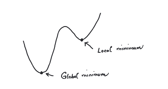
Graph of function defined on an interval. This function has a local minimum, which is not a global minimum.

Give an example of a local minimum that is not a global minimum for a precisely specified function. Also give an example of a global minimum, which is not uniquely defined (again for a precisely specified function). Uniquely defined means that there is precisely one $x_0$ , such that $f(x_0)$ is minimal.

We might as well have talked about maximum instead of minimum above.

Reformulate Definition 6.9 in order to define a local and a global maximum.

A local extremum is a point $x_0\in S$ , which is either a local minimum or a local maximum.

Convex functions $f: C\rightarrow \RR$ are interesting, because of the local nature of the minimization problem

$\minunder{x\in C}\; f(x) \tag{6.3}$

If you run into a local minimum in (6.3) , then you are sure that it also is a global minimum! This is the content of the result below.

Let $f: C\rightarrow \RR$ be a convex function defined on a convex subset $C\subseteq \RR^d$ . If $v_0\in C$ is a local minimum, then $v_0$ is a global minimum. If $f$ is strictly convex, then a global minimum for $f$ is unique.

By the definition of local minimum in Definition 6.9 , there exists $\epsilon > 0$ , such that $f(v_0)\leq f(v)$ , when $v \in C$ and $\abs{ v - v_0 }< \epsilon$ . Suppose that $v_0$ is not a global minimum. Then there exists $v_1\in C$ with $f(v_1) < f(v_0)$ . Consider the point

$v_t = (1 - t) v_0 + t v_1\in C,$ where $0 < t < 1$ . Then

$f(v_t) \leq (1-t) f(v_0) + t f(v_1) < (1-t) f(v_0) + t f(v_0) = f(v_0).$ Since $\abs{ v_t - v_0 } = t \abs{ v_1 - v_0 }$ , we can choose $t > 0$ sufficiently small such that $\abs{ v_t - v_0 } < \epsilon$ implying $f(v_0)\leq f(v_t)$ , since $v_0$ is a local minimum. This contradicts that $f(v_t) < f(v_0)$ for every $0 < t < 1$ . Let $f$ be strictly convex and let $v_0$ be a global minimum for $f$ . If $v_1\in C$ , $v_1\neq v_0$ and $f(v_1) = f(v_0)$ , then

$f((1-\lambda) v_0 + \lambda v_1) < (1-\lambda) f(v_0) + \lambda f(v_1) = f(v_0)$ for $0 < \lambda < 1$ . This would contradict the global minimality of $v_0$ , since $v_0\neq (1-\lambda)v_0 + \lambda v_1\in C$ for $0< \lambda < 1$ .

Which of the following statements are true?

A local minimum of a convex function is always a global minimum.

Every convex function $f:\RR\rightarrow \RR$ has a global minimum.

A strictly convex function has at most one global minimum.

The function $f(x) = a x + b$ with $a\neq 0$ is strictly convex.

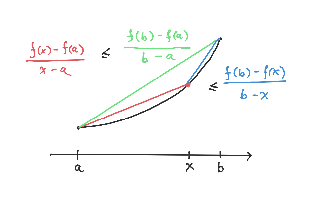
The following little result turns out to be very useful and also very intuitive and drawable! It is a key component in characterizing convex differentiable functions $f(x)$ in terms of $f''(x)$ . We will not give the proof here.

Let $f:[a,b]\rightarrow \RR$ be a convex function. Then

$\frac{f(x) - f(a)}{x - a} \leq \frac{f(b)-f(a)}{b - a} \leq \frac{f(b)-f(x)}{b - x}$ for $a < x < b$ .

The result in Lemma 6.15 is depicted above. A formal proof can be given from first principles only using Definition 4.26 .

6.3 Differentiable functions

To appreciate the depth of the notion of differentiability, you should read the story (joke, actually) in the second paragraph of section 8-2 in volume I of the famous Feynman Lectures on Physics. Below is a photograph of the master explainer in action.

6.3.1 Definition

Let $f:(a, b)\rightarrow \RR$ be a function defined on the open interval $(a, b)\subset \RR$ . What should it mean that $f$ is differentiable at a point $x_0\in (a, b)$ ? The whole idea fits in one sentence.

Zoom in on the graph at the point $(x_0, f(x_0))$ and it eventually looks like a line. The slope of that line is the derivative $f'(x_0)$ .

Try it yourself, right now. The cell below draws the graph of $f(x) = x^3$ together with a dashed line through the point $(1, 1)$ . Run it, then zoom in on the black point with the scroll wheel (or a trackpad pinch), or by dragging a small rectangle around it — keep zooming and watch the curve straighten into the dashed line. Double-click the plot to zoom all the way out again. (The first run downloads the plotting library, so it may take a little while.)

Live Python

import numpy as np
import plotly.graph_objects as go

f = lambda x: x**3      # try np.sin(1/x) around x0 = 0.1, np.exp(x), ...
x0 = 1.0                # the point to zoom in on

# slope at x0, computed numerically so any f works
c = (f(x0 + 1e-6) - f(x0 - 1e-6)) / 2e-6

# sample densely near x0, so the graph stays honest at any zoom level
h = np.geomspace(1e-7, 2.0, 4000)
x = np.concatenate([x0 - h[::-1], [x0], x0 + h])
with np.errstate(all="ignore"):
    y = f(x)            # singularities (like 1/x at 0) become gaps

# a steep tangent must not ruin the y axis: clip it to the vertical
# range of the graph itself (NaN cuts the line outside)
finite = y[np.isfinite(y)]
pad = 0.1 * (finite.max() - finite.min()) + 1e-12
ylo, yhi = finite.min() - pad, finite.max() + pad
t = f(x0) + c * (x - x0)
t[(t < ylo) | (t > yhi)] = np.nan

fig = go.Figure()
fig.add_trace(go.Scatter(x=x, y=y, mode="lines",
                         name="f(x)", line=dict(width=3)))
fig.add_trace(go.Scatter(x=x, y=t, mode="lines",
                         name="tangent", line=dict(dash="dash")))
fig.add_trace(go.Scatter(x=[x0], y=[f(x0)], mode="markers", name="x0",
                         marker=dict(size=9, color="black")))
fig.update_layout(dragmode="zoom", height=420,
                  margin=dict(l=40, r=20, t=30, b=40))
fig.show()

However far you zoom in, the graph of $x^3$ never stops looking like the dashed line through $(1, 1)$ — and the slope of that line is $f'(1) = 3$ . Zoom in around any other point and the curve straightens into a different line: the derivative depends on the point, which is why $f'$ is itself a function. The rest of this subsection turns the experience you just had into a precise definition.

Notice what did not happen in your zooming: nothing about the graph was changed — we only looked closer.

Now try the same experiment on a function with a corner. The cell below draws $f(x) = |x - 1|$ , which has a corner at the point $(1, 0)$ . Zoom in on the corner, as deep as you like. It never straightens: every zoom level shows the same V shape. There is no line that this graph eventually looks like, and $f$ is not differentiable at $1$ .

Live Python

So the intuition works, and it even detects corners. Let us now turn it into a precise definition — in three small steps.

Step 1: say what a zoom is. A zoom is a square window centered at the point $(x_0, f(x_0))$ : both axes show an interval of the same small half-width $w$ . Every zoom you performed above was such a window, with smaller and smaller half-width $w$ . The window must be a square because zooming has to treat both axes equally — stretching only one axis distorts the picture instead of enlarging it (more on this in the remark further below).

Step 2: blow the window up to standard size. Tiny windows are hard to compare, so we blow each one up, like enlarging a photograph. Blowing up divides every offset from the center by $w$ : a point on the graph with horizontal offset $t w$ (where $t\in [-1, 1]$ is the rescaled coordinate) and vertical offset $f(x_0 + t w) - f(x_0)$ lands at coordinates $t$ and

$g_w(t) = \frac{f(x_0 + t w) - f(x_0)}{w}.$ In other words: the blown-up window shows the graph of the function $g_w$ . The cell below draws these blown-up windows for three zoom levels, all in one frame, so that they can be compared directly. Watch the curves settle onto a line as $w$ shrinks. And try $f(x) = |x|$ at $x_0 = 0$ : the blow-ups are all identical — a corner looks like the same corner at every zoom level and never becomes a line.

Live Python

Step 3: say what must happen. "The graph becomes a line" now has an exact meaning: there is a slope $c$ , such that the curves $g_w$ settle onto the line $c\, t$ as $w\to 0$ . How far are we from the line? Writing $k = t w$ for the horizontal offset, a one-line computation gives, for $t\neq 0$ ,

$g_w(t) - c\, t = t\left(\frac{f(x_0 + k) - f(x_0)}{k} - c\right).$ Since $|t|\leq 1$ , everything hinges on the parenthesis. Give it a name:

$\epsilon(k) = \frac{f(x_0 + k) - f(x_0)}{k} - c.$ The curves settle onto the line exactly when $\epsilon(k) \to 0$ as $k\to 0$ — that is, when $\epsilon$ , extended by $\epsilon(0) = 0$ , is continuous at $0$ in the sense of the previous chapter. Finally, multiply the definition of $\epsilon$ by $k$ and rearrange:

$f(x_0 + k) = f(x_0) + c\, k + \epsilon(k)\, k.$ This single equation is the definition we were after — reached from the zoom picture, not decreed from above. The $\epsilon$ -function in it is nothing mysterious: it is the zoom error, recording how far the graph deviates from the line, relative to the zoom level.

The function $f: (a, b)\rightarrow \RR$ is differentiable at $x_0\in (a, b)$ if there exists

$c\in \RR$
$\delta > 0$ with $x_0 - \delta, x_0 + \delta\in (a, b)$ i.e., $a + \delta < x_0$ and $x_0< b-\delta$ .
A function $\epsilon: (-\delta, \delta) \rightarrow \RR$ continuous at $0$ with $\epsilon(0) = 0$ ,

such that

$f(x_0 + h) - f(x_0) = c h + \epsilon(h) h \tag{6.4}$ for every $h\in (-\delta, \delta)$ .

The number $c$ is denoted $f'(x_0)$ and called the derivative of $f$ at $x_0$ ; $f$ is called differentiable if it is differentiable at every $x_0\in (a, b)$ .

Chatbot Prompt

Please explain the definition of differentiability given below. Illustrate by a few example and quiz me afterwards. ''' The function $f: (a, b)\rightarrow \RR$ is differentiable at $x_0\in (a, b)$ if there exists \begin{enumerate}[(i)] \item $c\in \RR$ \item $\delta > 0$ with $x_0 - \delta, x_0 + \delta\in (a, b)$ i.e., $a + \delta < x_0$ and $x_0< b-\delta$. \item A function $\epsilon: (-\delta, \delta) \rightarrow \mathbb{R}$ continuous at $0$ with $\epsilon(0) = 0$, \end{enumerate} such that \begin{equation} f(x_0 + h) - f(x_0) = c h + \epsilon(h) h \end{equation} for every $h\in (-\delta, \delta)$.

The number $c$ is denoted $f'(x_0)$ and called \emph{the derivative} of $f$ at $x_0$; $f$ is called \emph{differentiable} if it is differentiable at every $x_0\in (a, b)$. '''

Definition 6.17 is the zoom picture written out. It also contains the classical description of the derivative: dividing (6.4) by $h$ gives

$\frac{f(x_0 + h) - f(x_0)}{h} = c + \epsilon(h),$ and the left hand side is the slope of the line through $(x_0, f(x_0))$ and the nearby point $(x_0 + h, f(x_0 + h))$ on the graph. So $\epsilon(h)\to 0$ says exactly that these slopes tend to $c$ i.e.,

$\lim_{h\to 0} \frac{f(x_0 + h) - f(x_0)}{h} = f'(x_0).$ This is how the derivative is often introduced — Newton would say that $f'(x_0)$ is the slope just before $x$ becomes $x_0$ — and you may use the limit description and the zoom picture interchangeably.

Two fine points about the zoom intuition. First, the window must be a square: plotting software often stretches the two axes independently, and with enough one-sided stretching almost any graph can be made to look flat. Honest zooming treats both axes equally. Second, "looks like a line" must mean a line with a slope $c\in \RR$ : zooming in on $f(x) = \sqrt[3]{x}$ at $x_0 = 0$ produces something that looks more and more like a vertical line — no real number describes that slope, and the function is not differentiable at $0$ , even though the zoomed picture straightens. Try f = lambda x: np.cbrt(x) with x0 = 0 in the cells above and watch the graph escape through the top and bottom of the window.

If a function $f:(a, b)\rightarrow \RR$ is differentiable, we get a new function $f':(a, b)\rightarrow \RR$ giving the (first) derivative at a point as output. We may ask again if this function is differentiable. If this is so, we may define a function $f'':(a, b)\rightarrow \RR$ given by $f''(x) = (f')'(x)$ called the second derivative. This procedure may be continued. We use the notation $f^{(n)}$ for the $n$ -th derivative.

Let us apply Definition 6.17 to the function $f(x) = x^2$ at the point $x_0$ . Here

$f(x_0 + h) - f(x_0) = (x_0 + h)^2 - x_0^2 = 2 x_0 h + h^2.$ Here you immediately see that $c = f'(x_0) = 2 x_0$ with $\epsilon(h) = h$ (and $\delta = \infty$ ) in Definition 6.17 .

Use Definition 6.17 to formally show that $f'(x) = 3 x^2$ if $f(x) = x^3$ .

A differentiable function is continuous as is shown in the following result.

If the function $f: (a, b)\rightarrow \RR$ is differentiable at $x_0\in (a, b)$ , then it is continuous at $x_0$ .

That $f$ is continuous at $x_0$ means (recall Definition 5.65 ) that to every $\epsilon > 0$ , we may find $\delta > 0$ so that

$| x - x_0 | < \delta \implies | f(x) - f(x_0) | < \epsilon. \tag{6.5}$ We are assuming that $f$ is differentiable at $x_0$ , so according to Definition 6.17 , there exists a number $c$ so that (with $h = x-x_0$ )

$| f(x) - f(x_0) | = |(c + \epsilon(x-x_0)) (x-x_0)|.$ I will not write every detail out here, but you can see from the formula above that $|f(x) - f(x_0)| < M | x - x_0 |$ for some number $M$ , when $|x - x_0|$ is sufficiently small. This gives a $\delta$ that can be used in (6.5) .

The ReLU function $f(x) = \max(0, x)$ is an example of a function, which is continuous, but not differentiable at $x_0 = 0$ . This is much related to its sharp corner there.

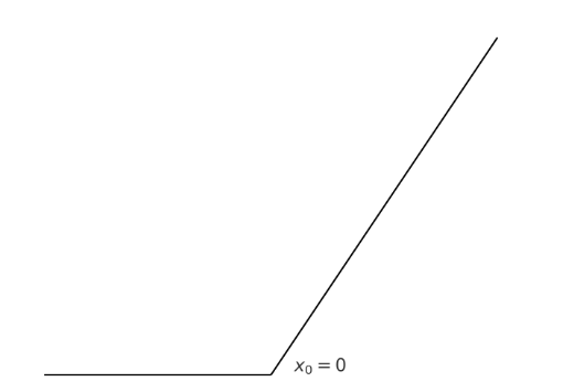As mentioned in these notes, the ReLU function plays a prominent role as an activation function in neural networks.

Show precisely that the ReLU function is not differentiable at $0$ .

6.3.2 Formulas

In operating with differentiable functions you are supposed to draw on your previous knowledge. I have summarized some of this knowledge below (even though we will give hints below as how to prove some of the rules).

If $f(x) = a g(x)$ , where $a\in \RR$ , then
$f'(x) = a g'(x).$
If $f(x) = x^n$ , where $n \in \NN$ , then
$f'(x) = n x^{n-1}.$
If $f(x) = e^x$ , then
$f'(x) = f(x) = e^x.$
If $f(x) = \log(x)$ , then
$f'(x) = 1/x.$ Here $\log(x)$ denotes the logarithm with base $e$ .
If $f(x) = \sin(x)$ , then
$f'(x) = \cos(x).$
If $f(x) = \cos(x)$ , then
$f'(x) = -\sin(x).$
If $f(x)$ and $g(x)$ are differentiable functions, then the derivative of their product is
$(f g)'(x) = f'(x) g(x) + f(x) g'(x).$
If $f(x)$ and $g(x)$ are differentiable functions, then the derivative of their quotient is
$\left(\frac{f(x)}{g(x)}\right)' = \frac{f'(x) g(x) - f(x) g'(x)}{g(x)^2}.$
If $f(x)$ and $g(x)$ are composable differentiable functions, then the derivative of their composite is
$(f\circ g)'(x) = f'(g(x)) g'(x).$

Suppose that $f(x) = \sin(x)$ . What is

$f^{(17)}(x)?$

6.3.3 The derivative of a product

From high school you know that the derivative of a product of two functions $f$ and $g$ is given by the formula

$(f g)'(x) = f'(x) g(x) + f(x) g'(x). \tag{6.6}$

We can use the $\epsilon$ -definition (6.4) to derive the product rule in (6.6) . The computation below is a bit cumbersome, but actually quite doable. We assume to begin with that $f$ and $g$ are differentiable at $x_0$ according to (6.4) i.e.,

$\begin{aligned} f(x_0 + h) &= f(x_0) + f'(x_0)h + \epsilon_f(h) h\\ g(x_0 + h) &= g(x_0) + g'(x_0)h + \epsilon_g(h) h.\\ \end{aligned}$ Then we start the computation:

$\begin{aligned} &(f g)(x_0 + h) = f(x_0 + h) g(x_0 + h) =\\ &(f(x_0) + f'(x_0)h + \epsilon_f(h) h)\,\, (g(x_0) + g'(x_0) h + \epsilon_g(h) h) =\\ &f(x_0) g(x_0) + (f'(x_0) g(x_0) + f(x_0) g'(x_0)) h + \epsilon(h) h, \end{aligned} \tag{6.7}$ where the function

$\epsilon(h) = f(x_0) \epsilon_g(h) + f'(x_0) g'(x_0) h + f'(x_0) \epsilon_g(h) h + \epsilon_f(h) g(x_0) + \epsilon_f(h) g'(x_0) h + \epsilon_f(h) \epsilon_g(h) h \tag{6.8}$ is seen to be continuous at $h=0$ with $\epsilon(0) = 0$ . The end result of this computation shows that $f g$ is differentiable at $x_0$ with

$(f g)'(x_0) = f'(x_0) g(x_0) + f(x_0) g'(x_0) \tag{6.9}$ again according to (6.4) .

Show that the $\epsilon$ function defined in (6.8) satisfies the relevant conditions in Definition 6.17 .

The formula for the derivative of a fraction i.e.,

$\left(\frac{f(x)}{g(x)}\right)' = \frac{f'(x) g(x) - f(x) g'(x)}{g(x)^2}$ can be derived using a neat little trick. This is the topic of the following exercise.

Show how the product rule may be used to derive the rule for finding the derivative of a fraction:

$\left(\frac{f}{g}\right)'(x_0) = \dfrac{f'(x_0) g(x_0) - f(x_0) g'(x_0)}{g(x_0)^2}.$

Hint

$f'(x) = \left(g(x) \left(\frac{f(x)}{g(x)}\right)\right)'.$

6.3.4 The one variable chain rule

The formula for the derivative of a composite function is given by

$(f\circ g)'(x_0) = f'(g(x_0)) g'(x_0),$ where $g(x_0)$ is in the domain of $f$ . Let us see how (6.4) applies in showing this.

Suppose that $f$ is differentiable at $g(x_0)$ and $g$ is differentiable at $x_0$ , then we can mess around a bit with the $\epsilon$ -functions for $f$ and $g$ for the composite function $f(g(x))$ around $x_0$ :

$\begin{aligned} f(g(x_0 + h)) &= f(g(x_0) + g'(x_0) h + h \epsilon_g(h))\\ &= f(g(x_0)) + f'(g(x_0)) g'(x_0) h + \epsilon(h) h, \end{aligned}$ where (take a deep breath)

$\epsilon(h) = f'(g(x_0)) \epsilon_g(h) + \epsilon_f\bigl(g'(x_0) h + \epsilon_g(h)h\bigr)\bigl(g'(x_0) + \epsilon_g(h)\bigr).$ Here $\epsilon$ is seen to be continuous at $0$ with $\epsilon(0)=0$ i.e., the composition $f(g(x))$ is differentiable at $x_0$ with derivative

$(f\circ g)'(x_0) = f'(g(x_0)) g'(x_0). \tag{6.10}$

The formula (6.10) is extremely important and useful. We give some applications in the exercises below.

For the function $f(x) = x^n$ for $n\in \NN$ , you already know that $f'(x) = n x^{n-1}$ . Show that if you define the function $g: \{x\in \RR \mid x > 0\} \rightarrow \RR$ by

$g(x) = x^a := e^{\log(x) a},$ for an arbitrary number $a\in \RR$ , then $g'(x) = a x^{a-1}$ .

Compute the derivative of the function $f: (0, \pi) \rightarrow \RR$ given by

$f(x) = \dfrac{1}{\sqrt{\sin(x)}}$ using only paper and pencil! You can check your result afterwards using a computer.

Suppose that $g$ and $f$ are inverse functions i.e.,

$f(g(x)) = x\qquad \text{and} \qquad g( f(x)) = x.$ If you know the derivative of $f$ , how can you use the chain rule to get the derivative of $g$ ? Illustrate with examples like $f(x) = x^2$ and $g(x) = \sqrt{x}$ , $f(x) = e^x$ and $g(x) = \log(x)$ .

Suppose that $f:\RR\rightarrow \RR$ is a convex function. We know that $f$ is continuous, but is $f$ differentiable at every point $x_0\in \RR$ ?

Hint

Nope. This is wrong. Come up with a convex function $f$ and a point $x_0$ , such that $f$ is not differentiable at $x_0$ .

6.3.5 The Newton-Raphson method for finding roots

We begin this section with a surprising example.

Suppose that $a> 0$ and we wish to compute $\sqrt{a}$ . To do this we may focus on the quadratic equation $f(x) = x^2 - a = 0$ and attempt to compute an approximate value $x_0\geq 0$ , such that $f(x_0)$ is close to $0$ . Let me at this point disclose that there is a very effective iterative scheme for doing this. You start by putting $x_0 = a$ and then iterate using the formula

$x_{i+1} = \frac{1}{2}\left(x_i + \frac{a}{x_i}\right) \tag{6.11}$ to get better and better approximations $x_0, x_1, x_2, \dots$ to $\sqrt{a}$ .

The formula in (6.11) is derived from

$x_{i+1} = x_i - \frac{f(x_i)}{f'(x_i)},$ where $f(x) = x^2 - a$ .

You can try out (6.11) below.

Live Python

I have been in complete awe of the Newton-Raphson method since my early youth. It is an algorithm, where the notion of differentiability really shines.

The method comes from Definition 6.17 with $h = x - x_0$ : we are assuming that $x_0$ is very close to $x$ , where $f(x) = 0$ . Then

$f(x) - f(x_0) = f'(x_0) (x- x_0) + \text{a very small number}.$ Ignoring the very small number and solving this equation for $x$ we get

$x = x_0 - \frac{f(x_0)}{f'(x_0)}.$

In the python cell below, I have entered the algorithm starting in $x_0 = 0$ running ten iterations for finding a zero for $f(x) = \cos(x) - x$ .

Graph

Live Python

Give an example, where the Newton-Raphson method cycles between points and never finds the desired zero. Perhaps a drawing will help here.

The Newton-Raphson converges rapidly in most cases. Of course, it breaks down violently if it runs into a critical point i.e., a point $x$ , such that $f'(x) = 0$ .

Below is some python code for experimenting with Newton's method.

Live Python

The formula (see button in Example 1.87 ) for the (monthly) payment $Y$ on a (car) loan over $N$ payments with a down payment of $P$ and an interest rate of $r$ (per payment or term) is given by the formula

$Y = \frac{r P}{1 - \left(\frac{1}{1+r}\right)^N}.$ There is no explicit formula for calculating $r$ given $Y, P$ and $N$ . Here the Newton-Raphson method is invaluable for estimating $r$ by approximating a zero for the function

$r(x) = Y - \frac{x P}{1 - \left(\frac{1}{1+x}\right)^N}.$

Your bank promises you a loan of $1.000.000$ DKK with yearly payments of $45.000$ DKK over $30$ years. At the same time it claims that its interest rate is very favorable at only $1.0$ %. Here the bank is wrong! What is the real interest rate? How much money do you save (compared to the original offer from the bank) if you insist that the bank offers you the promised interest rate of $1.0$ %?

Python: check your answer

Live Python

6.3.6 Critical points and extrema

A critical point for a differentiable function $f:(a, b)\rightarrow \RR$ is a point $x_0\in (a, b)$ with

$f'(x_0) = 0.$

The crucial result here is the following. It seems to date back to Fermat (see Fermat's theorem).

Let $f : (a, b)\rightarrow \RR$ be a differentiable function. If $x_0$ is a local extremum for $f$ , then $x_0$ is a critical point i.e., $f'(x_0) = 0$ .

Suppose that $\xi$ is a local maximum and that

$f(\xi + h) - f(\xi) = f'(\xi) h + \epsilon(h) h$ according to (6.4) . If $f'(\xi)>0$ , then we can choose $\delta >0$ sufficiently small, such that $\abs{ \epsilon(h) } < f'(\xi)$ if $0\leq h < \delta$ , since $\epsilon(0) = 0$ and $\epsilon$ is continuous in $0$ . Therefore

$f(\xi + h) - f(\xi) = (f'(\xi) + \epsilon(h)) h > 0,$ contradicting that $\xi$ is a local maximum. The proof is similar for $f'(\xi) < 0$ and if $\xi$ is a local minimum.

Is the converse of the above lemma true i.e., if $f'(x_0) = 0$ is $x_0$ a local extremum?

Which of the following statements are true?

If $x_0$ is a local extremum of a differentiable function $f$ , then $f'(x_0) = 0$ .

If $f'(x_0) = 0$ for a differentiable function $f$ , then $x_0$ is a local extremum.

The ReLU function $f(x) = \max(0, x)$ is differentiable at every point of $\RR$ .

If $f'(x) > 0$ for every $x\in (a, b)$ , then $f$ is strictly increasing on $(a, b)$ .

Theorem 6.40 below is called the mean value theorem. It is a consequence of Lemma 6.37 and the extremely important Theorem 5.84 about continuous functions on compact subsets attaining their maxima and minima!

Let $f:[a, b]\rightarrow \RR$ be continuous and differentiable on $(a, b)$ . Then there exists $x_0\in (a, b)$ such that

$f'(x_0) = \frac{f(b) - f(a)}{b - a}.$

6.3.7 Increasing functions

The definition below is much simpler than the definition of differentiability.

A function $f:S\rightarrow \RR$ with $S\subseteq \RR$ is called increasing if

$x\leq y\Rightarrow f(x) \leq f(y)$ and strictly increasing if

$x< y\Rightarrow f(x) < f(y)$ for $x, y\in S$ .

Chatbot Prompt

Explain the definition below to me. Give some examples and test me. \begin{definition} A function $f:S\rightarrow \mathbb{R}$ with $S\subseteq \mathbb{R}$ is called
  \emph{increasing} if
  \begin{equation*}
    x\leq y\Rightarrow f(x) \leq f(y)
  \end{equation*}
  and \emph{strictly increasing} if 
  \begin{equation*}
    x< y\Rightarrow f(x) < f(y)
  \end{equation*}
  for $x, y\in S$.
\end{definition}

Give an example of an increasing function. Give an example of an increasing function that is not strictly increasing.

The following very important result is a consequence of Theorem 6.40 . You probably already know this result from your previous (danish) education (monotoniforhold!).

Let $f : (a, b)\rightarrow \RR$ be a differentiable function. Then $f$ is increasing if and only if $f'(x)\geq 0$ for every $x\in (a, b)$ . If $f'(x)> 0$ for every $x\in (a, b)$ , then $f$ is strictly increasing.

Which of the properties below are true for the function $f:\RR\rightarrow \RR$ given by

$f(x) = x^3+ 2 x^2 + x + 1?$

It has a global minimum.

It is differentiable.

It has three zeros.

It has exactly one critical point.

It is increasing.

It is continuous.

It is convex.

It has a local minimum.

It has a local maximum.

Show that $f(x) = x^3$ is strictly increasing i.e.,

$x < y \implies x^3 < y^3.$ Hint

$y^3 - x^3 = (y - x) (y^2 + x y + x^2),$ but why is $y^2 + x y + x^2$ always $> 0$ except when $x = y = 0$ ?

Suppose that $f: [a, b] \rightarrow \RR$ is a continuous function, such that $f$ is differentiable on the open interval $(a, b)$ . Is $f$ increasing on $[a, b]$ if $f'(x)\geq 0$ for every $x\in (a, b)$ ?

Is it possible for a strictly increasing function $f: \RR \rightarrow \RR$ to be bounded i.e., does there exist a (positive) number $M$ , such that $|f(x)| \leq M$ for every $x\in \RR$ ?

Hint

Have a look at

$f(x) = \dfrac{1}{1 + e^{-x}}.$

6.4 Taylor polynomials

If $x_0$ is a critical point for $f$ we cannot conclude that $x_0$ is a local extremum. We know that $f'(x_0)=0$ and we can get more information out of $f$ by exploring the signs of

$f''(x_0), f'''(x_0), \dots$

Suppose that

$f(x) = a_0 + a_1 x + a_2 x^2 + \cdots + a_n x^n$ is a polynomial, then

$f(x) = f(0) + f'(0) x + \frac{f''(0)}{2} x^2 + \cdots + \frac{f^{(n)}(0)}{n!} x^n. \tag{6.12}$

For nice functions like $f(x) = e^x$ we can play this game ad infinitum. In fact in this way we get the beautiful infinite series

$e^x = 1 + x + \frac{x^2}{2} + \frac{x^3}{6} + \cdots + \frac{x^n}{n!} + \cdots.$

If $f$ is an $n$ times differentiable function defined at $0$ , we call the polynomial in (6.12) the Taylor polynomial about the point $0$ of degree $n$ associated with $f$ . Similarly, one may also define the Taylor polynomial of order $n$ about a point $a$ by

$f(a) + f'(a) (x-a) + \frac{f''(a)}{2} (x-a)^2 + \cdots + \frac{f^{(n)}(a)}{n!} (x-a)^n.$ Taylor polynomials can be used to approximate more complicated functions such as $\cos(x)$ and $\sin (x)$ with a well defined error term. This is cool classical mathematics. Unfortunately we do not have time to go deeper into Taylor's theorem, which states this in precise terms.

You can watch the approximation happen in the cell below: the Taylor polynomials of $\sin(x)$ hug the graph on a wider and wider interval as the degree grows. Change $f$ , the degrees, or the plotting window — and use the cell to check your answer to the exercise below.

Live Python

Compute the Taylor polynomial for $f(x) = \cos(x)$ up to degree $10$ .

Suppose you have a number $i$ that satisfies

$i^2 = -1.$ Can you make sense of the formula

$e^{i x} = \cos(x) + i \sin(x)$ using Taylor polynomials?

In the context of optimization, the following result becomes important. We will not give the proof, but only notice that Theorem 6.40 also here plays an important role.

Let $x_0$ be a critical point of an $n+1$ times differentiable function $f:(a, b)\rightarrow \RR$ , such that $f^{(n+1)}$ is a continuous function,

$\begin{aligned} f''(x_0) &= 0\\ f'''(x_0) &= 0\\ &\vdots\\ f^{(n-1)}(x_0) &= 0 \end{aligned}$ and $f^{(n)}(x_0)\neq 0$ . If $n$ is even, then $x_0$ is a local minimum if $f^{(n)}(x_0) > 0$ and a local maximum if $f^{(n)}(x_0)<0$ . If $n$ is odd, then $x_0$ is not a local extremum.

Let us apply Theorem 6.50 to the function

$f(x) = a x^2 + b x + c,$ where $a\neq 0$ . Here $f'(x) = 2 a x + b$ and

$x_0 = - \frac{b}{2 a}$ is a critical point (why?). Since

$f''(x_0) = 2 a,$ we see that $x_0$ is a local minimum if $a > 0$ and a local maximum if $a < 0$ .

Have you seen Example 6.51 elsewhere, perhaps in a more geometric setting? What type of curve is the graph of $f(x)$ ? Here you may consult your previous mathematical knowledge.

What is the outcome, when you apply Theorem 6.50 to the function $f(x) = x^3$ at $x_0 = 0$ ?

Show that $x_0=0$ is a critical point of the function $f: (-\frac{1}{2}, \infty)\rightarrow \RR$ defined by

$f(x) = e^x + \log(1 + 2 x) - 3 x.$ Use Theorem 6.50 in deciding if it is a local maximum or minimum or neither.

6.5 Differentiable convex functions

The following theorem is proved using Lemma 6.15 and Theorem 6.40 . It immediately implies Corollary 6.55 , which is the result mostly used.

Let $f:(a, b)\rightarrow \RR$ be a differentiable function. Then $f$ is convex if and only if $f'$ is increasing. If $f'$ is strictly increasing, then $f$ is strictly convex.

Theorem 6.54 leads to the following all important result.

Let $f:(a, b)\rightarrow \RR$ be a twice differentiable function. Then $f$ is convex if and only if $f''(x)\geq 0$ for every $x\in (a, b)$ . If $f''(x) > 0$ for every $x\in (a, b)$ , then $f$ is strictly convex.

Wait! Stop! Why did I not write $f''(x) > 0$ if and only if $f$ is strictly convex?

Which of the properties below are true for the function $f(x) = x^3$ ?

It is strictly convex on $[0, 1]$ .

Since $f'(0) = 0$ , it must have a local minimum for $x=0$ .

It is convex on $[0, 1]$ .

It is convex on $(-1, 1)$ .

It is strictly convex on $(0, 1]$ .

You cannot deduce from Corollary 6.55 that the function $g: \RR \rightarrow \RR$ given by $g(x) = x^4$ is a strictly convex function. Why not?

You can deduce from Corollary 6.55 that $f(x) = x^2$ is a strictly convex function. How can $g(x) = f(x)^2$ be used to prove that $g(x)$ is a strictly convex function?

Show that $f(x) = e^x$ is a strictly convex function $f: \RR\rightarrow \RR$ .

Show that $f(x) = -\log(x)$ is a strictly convex function $f: (0, \infty) \rightarrow \RR$ .

Show that $f: \{x\in \RR \mid x \geq 0\}\rightarrow \RR$ given by

$f(x) = -\sqrt{x}$ is a strictly convex function.

Another nice application of Lemma 6.15 (and Theorem 6.54 ) is the following.

Let $f:(a, b)\rightarrow \RR$ be a differentiable function. Then $f$ is convex if and only if

$f(y) \geq f(x) + f'(x)(y-x)$ for every $x, y\in (a, b)$ .

Python: the graph sits above its tangents

Theorem 6.61 says that a differentiable function is convex exactly when its graph lies above every one of its tangent lines. The cell below draws a function with four of its tangents. For a convex function no tangent ever crosses the graph. Try f = lambda x: x**3 and watch a tangent cut through.

Live Python

Suppose that $f:(a, b)\rightarrow \RR$ is a differentiable convex function and $x_0\in (a, b)$ is a critical point for $f$ . What can you say about $x_0$ using Theorem 6.61 ?