7 Several variables

A function of several variables usually refers to a function

$f: \RR^d \rightarrow \RR, \tag{7.1}$ where $d > 1$ is a natural number. We have already seen functions of several variables with $d>1$ . In particular, in Chapter 4 , we saw linear functions (in connection with linear programming) like

$f(x_1, x_2) = 3 x_1 + 2 x_2. \tag{7.2}$ This is a rather simple function of several variables with $d=2$ in (7.1) . In general functions as in (7.1) can be wildly complicated. One of the main purposes of this chapter is to zero in on the class of differentiable functions in (7.1) . In Chapter 6 we defined what it means for a function of one variable to be differentiable. This was inspired by zooming in at a point on the graph of the function. In several variables (for $n > 1$ ) one has to be a bit clever in the definition of differentiability. The upshot is that the derivative at a point now is a row vector (or more generally a matrix) instead of being a single number. As an example, using notation that we introduce in this chapter, the derivative of the function in (7.2) at $(0, 0)$ is

$\left(\pd{f}{x_1}\quad \pd{f}{x_2}\right) = \left(3\quad 2\right).$ This notation means that partial differentiation with respect to a variable occurs i.e., one fixes the variable and computes the derivative with respect to this variable viewing all the other variables as constants.

First some treasured memories from the author's past.

7.1 Introduction

Many years ago (1986-89), I had a job as a financial analyst in a bank (now a hotel!) working (often late at night) with a spectacular view of Copenhagen from the office circled below.

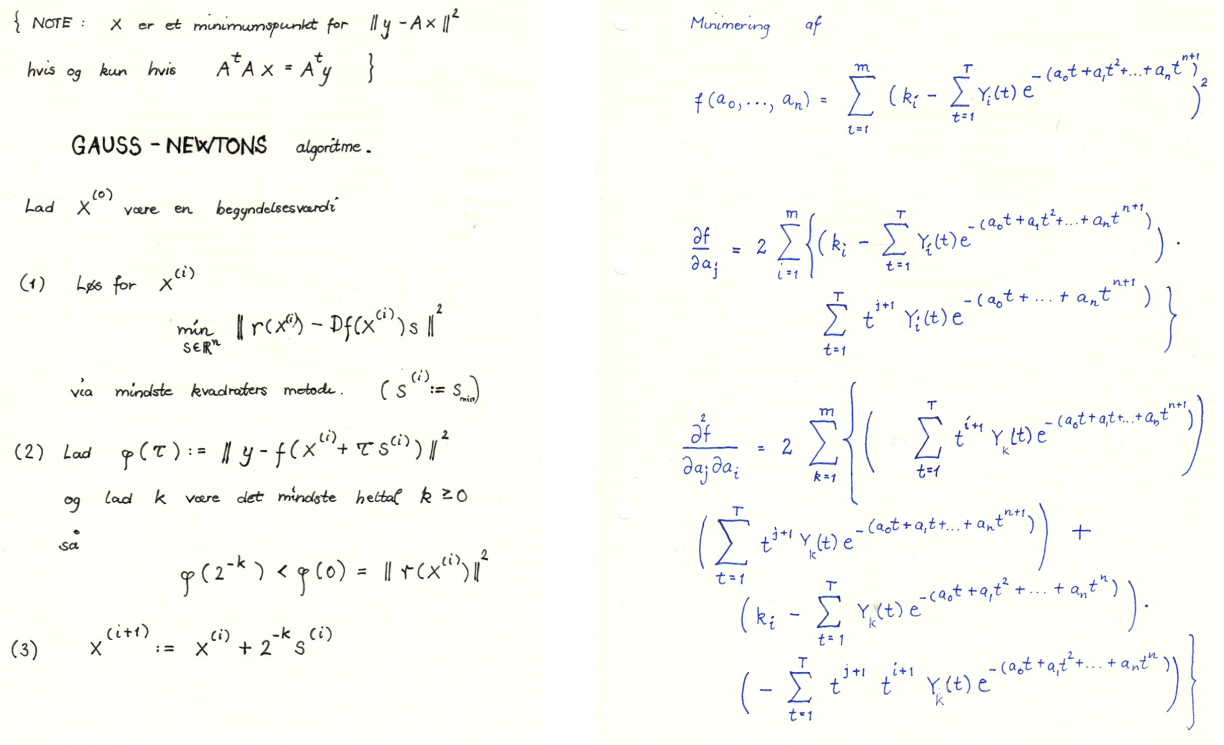
This was long before a financial analyst became a quant and machine learning became a buzz word. Digging through my old notes from that time, I found the outlines below.

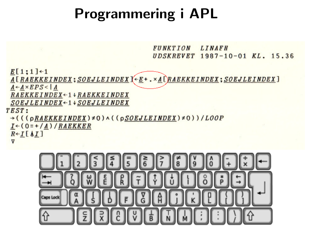
These were notes I made in connection with modelling the yield curve for zero coupon bonds. I had to fit a very non-linear function in several variables to financial data and had to use effective numerical tools (and programming them ¹

in APL). Tools that are also used today in machine learning and data science.

Ultimately we are interested in solving optimization problems like

$\minunder{(x_1, \dots, x_d)\in C}\; f(x_1, \dots, x_d),$ where $C\subseteq \RR^d$ and $f:\RR^d\rightarrow \RR$ is a differentiable (read nice for now) function.

Training neural networks is a fancy name for solving an optimization problem, where usually $C = \RR^d$ and $f$ is built just like in the least squares method from some data points. The difference is that in neural networks, $f$ is an incredibly complicated (differentiable) function composed of several intermediate functions. We do not, as in the method of least squares, have an explicit formula for finding a minimum. We have to rely on iterative methods. One such method is called gradient descent. By the end of this chapter, in Section 7.9 , you will use it to train genuine neural networks — from a single neuron to a network reading handwritten digits and, at the very end, one that writes — live in these notes.

Recall the definition of a function $f:\RR\rightarrow \RR$ being differentiable at a point $x_0\in \RR$ with derivative $c = f'(x_0)$ . Here we measured the change $f(x_0+h) - f(x_0)$ of $f$ in terms of the change $h$ (in $x$ ). It had to have the form

$f(x_0+h) - f(x_0) = c\, h + \epsilon(h) h, \tag{7.3}$ where $\epsilon:(-\delta, \delta)\rightarrow \RR$ is a function continuous in $0$ with $\epsilon(0) = 0$ and $\delta>0$ small. If you divide both sides of (7.3) by $h$ you recover the usual more geometric definition of differentiability as a limiting slope:

$\lim_{h\to 0}\, \frac{f(x_0 + h) - f(x_0)}{h} = c = f'(x_0). \tag{7.4}$

We wish to define differentiability at $v_0\in \RR^d$ for a function $f: \RR^d\rightarrow \RR^m$ . In this setting the quotient

$\frac{f(v_0 + h) - f(v_0)}{h}$ in (7.4) does not make any sense. There is no way we can divide a vector $f(v_0 + h) - f(v_0)\in \RR^m$ by a vector $h\in \RR^d$ , unless of course $m = d = 1$ as in (7.4) , where we faced usual numbers.

The natural thing here is to generalize the definition in (7.3) . First let us recall what functions $f:\RR^d\rightarrow \RR^m$ look like.

7.2 Vector functions

We will flesh out the general Definition 1.104 in a special case below.

A function $f:\RR^d\rightarrow \RR^m$ takes a vector $(x_1, \dots, x_d)\in \RR^d$ as input and gives a vector $(y_1, \dots, y_m)\in \RR^m$ as output. This means that every coordinate $y_1, \dots, y_m$ in the output must be a function of $x_1, \dots, x_d$ i.e.,

$y_i = f_i(x_1, \dots, x_d)$ for $i = 1, \dots, m$ . So in total, we may write $f$ as

$f(x_1, \dots, x_d) = \begin{pmatrix} f_1(x_1, \dots, x_d)\\ \vdots \\ f_m(x_1, \dots, x_d) \end{pmatrix}. \tag{7.5}$

Each of the (coordinate) functions $f_i$ are functions from $\RR^d$ to $\RR$ .

Look back at Exercise 1.125 . Write down precisely the vector function $h:\RR^2\rightarrow \RR^2$ occurring there.

The function $f:\RR^2\rightarrow \RR^2$ is rotating a vector $90$ degrees counter clockwise. What are $f_1$ and $f_2$ in

$f(x, y) = \begin{pmatrix} f_1(x, y)\\ f_2(x, y) \end{pmatrix}?$ Hint

Try rotating some specific vectors like $(1, 0), (0, 1), (1, 1)$ $90$ degrees. Do you see a pattern?

7.3 Differentiability

The definition of differentiability for a function $f:\RR^d\rightarrow \RR^m$ mimics (7.3) , except that $\epsilon(h) h$ is replaced by $\epsilon(h) |h|$ . Also the open interval $(a, b)$ is replaced by an open subset $U$ and the (open) interval $(-\delta, \delta)$ is replaced by an open subset $O$ containing $0$ .

Notice, however, that now the derivative is a matrix!

Let $f:U\rightarrow \RR^m$ be a function with $U\subseteq \RR^d$ an open subset. Then $f$ is differentiable at $v_0\in U$ if there exists

an $m\times d$ matrix $C$ ,
an open subset $O\subseteq \RR^d$ with $0\in O$ , such that $v_0+h\in U$ for every $h\in O$ ,
a function $\epsilon: O\rightarrow \RR^m$ continuous at $0$ with $\epsilon(0) = 0$ ,

such that

$f(v_0 + h) - f(v_0) = C\, h + \epsilon(h)\, \abs{ h },$ In this case, the $m\times d$ matrix $C$ is called the (matrix) derivative of $f$ at $v_0$ and denoted by $f'(v_0)$ .

The function $f$ is called differentiable if it is differentiable at every $v\in U$ .

For one variable we saw that differentiability at $x_0$ means that the graph looks like a line when you zoom in around $(x_0, f(x_0))$ . Definition 7.3 says the same thing one dimension up: for a function $f:\RR^2\rightarrow \RR$ the graph $z = f(x, y)$ is a surface in $\RR^3$ , the derivative is a $1\times 2$ matrix $C = (a\ b)$ , and $z = f(v_0) + C h$ describes a plane --- the tangent plane at $v_0 = (x_0, y_0)$ . Differentiability at $v_0$ means: zoom in on the point and the surface becomes indistinguishable from this plane.

You can watch this happen in the live cell below. The graph of $f(x, y) = x^3 - 3 x y^2$ is drawn in blue together with its tangent plane at the black point, shown as a red grid. Run the cell and drag the slider to shrink the window around the point --- the curved blue surface flattens into the red grid. Rotate the picture with the mouse to see it from all sides.

Live Python

import numpy as np
import plotly.graph_objects as go

f = lambda x, y: x**3 - 3*x*y**2   # try your own function
x0, y0 = 1.0, 0.5                  # the point to zoom in on

# the two slopes in C = (a b), computed numerically so any f works
e = 1e-6
a = (f(x0 + e, y0) - f(x0 - e, y0)) / (2*e)
b = (f(x0, y0 + e) - f(x0, y0 - e)) / (2*e)

red = [[0, "red"], [1, "red"]]
frames = []
for w in [2.0, 1.0, 0.5, 0.2, 0.1, 0.05, 0.02]:
    u = np.linspace(-w, w, 40)
    X, Y = np.meshgrid(x0 + u, y0 + u)
    Z = f(X, Y)
    T = f(x0, y0) + a*(X - x0) + b*(Y - y0)   # the tangent plane
    zlo = min(Z.min(), T.min()); zhi = max(Z.max(), T.max())
    pad = 0.05*(zhi - zlo) + 1e-9
    scene = dict(xaxis=dict(range=[x0 - w, x0 + w]),
                 yaxis=dict(range=[y0 - w, y0 + w]),
                 zaxis=dict(range=[zlo - pad, zhi + pad]),
                 aspectmode="cube")
    frames.append(go.Frame(
        name=f"{2*w:g}",
        data=[go.Surface(x=X, y=Y, z=Z, showscale=False,
                         colorscale="Blues"),
              go.Surface(x=X, y=Y, z=T, showscale=False,
                         colorscale=red, opacity=0.35,
                         # graph-paper grid, so the plane reads as a plane
                         contours=dict(
                             x=dict(show=True, color="darkred",
                                    width=3, size=w/4),
                             y=dict(show=True, color="darkred",
                                    width=3, size=w/4))),
              go.Scatter3d(x=[x0], y=[y0], z=[f(x0, y0)],
                           mode="markers", showlegend=False,
                           marker=dict(size=4, color="black"))],
        layout=dict(scene=scene)))

steps = [dict(method="animate", label=fr.name,
              args=[[fr.name], dict(mode="immediate",
                                    frame=dict(duration=0, redraw=True))])
         for fr in frames]

fig = go.Figure(data=frames[0].data, frames=frames)
fig.update_layout(scene=frames[0].layout.scene,
                  sliders=[dict(steps=steps, active=0,
                                currentvalue=dict(prefix="window: "))],
                  height=540, margin=dict(l=0, r=0, t=30, b=0))
fig.show()

For a taste of what non-differentiable looks like, try the ice cream cone $f(x, y) = \sqrt{x^2 + y^2}$ at the point $(0, 0)$ : the cone looks exactly the same at every zoom level --- its tip never flattens into a plane, no matter how far you drag the slider.

How do we compute the matrix derivative $C$ in the above definition? We need to look at the representation of $f$ in (7.5) and introduce the partial derivatives.

7.3.1 Partial derivatives

A function of one variable $x$ has a derivative with respect to $x$ . For a function of several variables $x_1, \dots, x_d$ we have a well defined derivative with respect to each of these variables. These are called the partial derivatives (if they exist) and they are defined below.

Let $f: U\rightarrow \RR$ be a function, where $U$ is an open subset of $\RR^d$ . Fix a point $v = (a_1, a_2, \dots, a_d)\in U$ and let

$p_i = f(a_1, \dots, a_{i-1}, x, a_{i+1}, \dots, a_d)$ for $i = 1, \dots, d$ . If $p_i$ is differentiable at $x = a_i$ according to Definition 6.17 (recalled in (7.3) ), then we say that the partial derivative of $f$ with respect to $x_i$ exists at $v\in U$ and use the notation

$\frac{\partial f}{\partial x_i}(v) := p_i'(a_i).$

The partial derivative with respect to a specific variable is computed by letting all the other variables appear as constants.

To get a feeling for the definition and computation of partial derivatives, take a look at the example below, where we compute using the classical (geometric) definition of the one variable derivative.

Consider the function $f: \RR^2 \rightarrow \RR$ given by

$f(x_1, x_2) = x_1 x_2^2 + x_1.$ Then

$\begin{aligned} \frac{\partial f}{\partial x_2}(v) &= \lim_{\delta\to 0}\frac{f(x_1, x_2 + \delta) - f(x_1, x_2)}{\delta}\\ & = \lim_{\delta\to 0} \frac{x_1 (x_2+\delta)^2 + x_1 - (x_1 x_2^2 + x_1)}{\delta}\\ &= x_1 \lim_{\delta\to 0}\frac{(x_2+\delta)^2 - x_2^2}{\delta} = x_1\, \lim_{\delta\to 0} (2 x_2 + \delta) = 2 x_1 x_2, \end{aligned}$ where $v = (x_1, x_2)$ . This example illustrates that $\frac{\partial f}{\partial x_i}$ can be computed just like in the one variable case, when the other variables ( $\neq x_i$ ) are treated as constants. Notice that

$\frac{\partial}{\partial x_1}\frac{\partial f}{\partial x_2} = \frac{\partial }{\partial x_2}\frac{\partial f}{ \partial x_1} = 2 x_2.$

Partial derivatives behave almost like the usual derivatives of one variable functions. You simply fix one variable that you consider the "real" variable and treat the other variables as constants.

$\frac{\partial}{\partial x}\left( \sin(x y) + x^2 y^2 + y\right) = y \cos(x y) + 2 x y^2.$

Below are examples of python code computing partial derivatives. Notice that the variables must be declared first.

Live Python

The computations above point to a really surprising result. It seems that it makes no difference if you compute the partial derivative with respect to $x_1$ and then with respect to $x_2$ or the other way around. You could, just for fun, try this out on the more complicated function

$f(x_1, x_2) = x_1 x_2^2 + \cos(\sin(x_1 x_2) + \log(x_1^{17} x_2)).$ This result is formulated in Theorem 7.11 below.

Use the python cell above to verify the computation of the partial derivative in Example 7.7 .

The following result tells us how to compute the matrix derivative.

Let $f:U\rightarrow \RR^m$ be a function with $U\subseteq \RR^d$ an open subset. If $f$ is differentiable at $v_0\in U$ , then the partial derivatives

$\frac{\partial f_i}{\partial x_j}(v_0)$ exist for $i = 1, \dots, m$ and $j = 1, \dots, d$ and the matrix $C$ in Definition 7.3 is

$C = \begin{pmatrix} \dfrac{\partial f_1}{\partial x_1}(v_0) & \cdots & \dfrac{\partial f_1}{\partial x_d}(v_0)\\ \vdots & \ddots & \vdots \\ \dfrac{\partial f_m}{\partial x_1}(v_0) & \cdots & \dfrac{\partial f_m}{\partial x_d}(v_0) \end{pmatrix}.$

The $j$ -th column in $C$ is $C e_j$ . Putting $h = \delta e_j$ for $\delta\in \RR$ in Definition 7.3 gives

$f(v_0 + \delta e_j) - f(v_0) = \delta C e_j + \epsilon(\delta e_j) \abs{ \delta }.$ The $i$ -th coordinate of this identity of $m$ -dimensional vectors can be written

$f_i(v_0 + \delta e_j) - f_i(v_0) = \delta C_{i j} + \tilde{\epsilon}_i(\delta) \delta \tag{7.6}$ where

$\tilde{\epsilon}_i(\delta) = \begin{cases} \epsilon_i(\delta e_j) \dfrac{\abs{ \delta }}{\delta} &\text{if } \delta\neq 0 \\ 0 &\text{if } \delta = 0 \end{cases}$ and (7.6) shows that $C_{ij} = \frac{\partial f_i}{\partial x_j}(v_0)$ .

Compute the matrix derivative of the vector function in Exercise 7.2 .

For a function $f:U\rightarrow \RR$ with $U\subseteq \RR^d$ an open subset, the partial derivative, if it exists for every $x\in U$ , is a new function

$\frac{\partial f}{\partial x_j} : U\rightarrow \RR.$ We will use the notation

$\frac{\partial^2 f}{\partial x_i \partial x_j} :=\frac{\partial}{\partial x_i} \frac{\partial f}{\partial x_j}$ for the iterated (second order) partial derivative.

The first part of following result is a converse to Proposition 7.9 . The second part contains the surprising symmetry of the second order partial derivatives under rather mild conditions. We will not go into the proof of this result, which is known as Clairaut's theorem.

Let $f:U\rightarrow \RR^m$ be a function with $U\subseteq \RR^d$ an open subset. If the partial derivatives for $f$ exist at every $x\in U$ with

$\frac{\partial f_i}{\partial x_j}$ continuous (for $i = 1, \dots, m$ and $j = 1, \dots, d$ ), then $f$ is differentiable. If the second order partial derivatives exist for a function $f : U\rightarrow \RR$ and are continuous functions, then

$\frac{\partial^2 f}{\partial x_i \partial x_j} = \frac{\partial^2 f}{\partial x_j \partial x_i}$ for $i, j = 1, \dots, d$ .

Verify (by hand!) the symmetry of the second order partial derivatives for the function $f$ in Example 7.7 i.e., show that

$\frac{\partial^2 f}{\partial x \partial y} = \frac{\partial^2 f}{\partial y \partial x}.$

Verify that $f: \RR^2\rightarrow \RR$ given by

$f(x, y) = \frac{x^2 y}{1 + y^2}$ is a differentiable function by computing

$\frac{\partial f}{\partial x}\qquad\text{and}\qquad\frac{\partial f}{\partial y}$ and applying Theorem 7.11 . Check also that

$\frac{\partial^2 f}{\partial x \partial y} = \frac{\partial^2 f}{\partial y \partial x}.$

7.4 Newton-Raphson in several variables!

There is a beautiful generalization of the Newton-Raphson method to several variable functions $f:\RR^d\rightarrow \RR^d$ . Consider first that you would like to solve the system

$\begin{aligned} y^2-x^3 + x &= 0\\ y^3-x^2 &= 0 \end{aligned}\tag{7.7}$ of non-linear equations in the two variables $x$ and $y$ . Notice that we are talking non-linear here. This is so much more difficult than the systems of linear equations that you encountered in a previous chapter.

However, just like we used Newton's method in one variable for solving a non-linear equation, Newton's method for finding a zero for a function $f: \RR^d\rightarrow \RR^d$ generalized to the iterative scheme

$v_{i+1} = v_i - f'(v_i)^{-1} f(v_i) \tag{7.8}$

provided that the $d\times d$ matrix derivative $f'(v_i)$ is invertible.

The reason that (7.8) works comes again from the powerful definition of differentiability in Definition 7.3 using that

$f(v) - f(v_0)\qquad \text{is close to}\qquad f'(v_0) (v - v_0) \tag{7.9}$ provided that $h = v - v_0$ is small. In fact, you get (again) (7.8) from (7.9) by putting $f(v)$ to $0$ , replacing is close to by $=$ and then isolating $v$ .

For the equations in (7.7) , the iteration scheme (7.8) becomes

$\begin{pmatrix} x_{i+1} \\ y_{i+1} \end{pmatrix} = \begin{pmatrix} x_i\\ y_i \end{pmatrix} - \begin{pmatrix} - 3 x_i^2+1 & 2 y_i\\ -2 x_i & 3 y_i^2 \end{pmatrix}^{-1} \begin{pmatrix} y_i^2-x_i^3 + x_i\\ y_i^3 - x_i^2 \end{pmatrix}. \tag{7.10}$

Verify the claim in (7.10) by applying (7.8) to

$f(x, y) = \begin{pmatrix} y^2 - x^3 + x\\ y^3 - x^2 \end{pmatrix}.$ Carry out sufficiently many iterations starting with the vector $(1, 1)$ in (7.10) to see the iteration stabilize. You should do this using a computer, for example by modifying the python code in the last half of Example 7.16 .

7.5 Local extrema in several variables

For a function $f:U\rightarrow \RR$ , where $U\subseteq \RR^d$ , the derivative $f'(v)$ at $v\in U$ is called the gradient for $f$ at $v$ . Classically, it is denoted $\nabla f(v)$ i.e.,

$\nabla f(v) = \left(\frac{\partial f}{\partial x_1}(v) \dots \frac{\partial f}{\partial x_d} (v)\right).$ The definition below is inspired by the one variable case (see Definition 6.36 ).

Let $f:U\rightarrow \RR$ be a function, where $U\subseteq \RR^d$ is an open subset. Suppose that the partial derivatives exist at $v_0\in U$ . Then $v_0$ is called a critical point for $f$ if $\nabla f(v_0)=0$ .

Consider the function $f: \RR^2 \rightarrow \RR^2$ given by

$f\begin{pmatrix} x \\ y \end{pmatrix} = \begin{pmatrix} 2 x + 3 \log(y)\\ 3 x / y - 3 y^2 \end{pmatrix}$ corresponding to finding critical points for the function

$g(x, y) = x^2 + 3 x \log(y) - y^3. \tag{7.11}$

You can left click and hold the graph computed below (after it has rendered) and rotate the surface to get a feeling for what (7.11) looks like. Zooming in is also possible.

Live Python

Here

$f' = \begin{pmatrix} 2 & 3/y \\ 3/y & -3 x/y^2 - 6 y \end{pmatrix}.$

In the python code below, Newton's method is started at $(1, 1)$ and iterated four times.

Live Python

If $v_0$ is not a critical point for $f$ we can use the gradient vector to move in a direction making $f$ strictly smaller/larger. This is very important for optimization problems.

Let $f: U\rightarrow \RR$ be a differentiable function, where $U\subseteq \RR^d$ is an open subset. Suppose that $u\in \RR^d$ and $\nabla f(v_0) u < 0$ for $v_0\in U$ . Then

$f(v_0 + \lambda u) < f(v_0)$ for $\lambda > 0$ small.

By the differentiability of $f$ ,

$f(v_0 + u) - f(v_0) = \nabla f(v_0) u + \epsilon(u) |u|,$ where $\epsilon:\RR^d \rightarrow \RR$ is a function satisfying $\epsilon(h) \rightarrow 0$ for $h\rightarrow 0$ . For $\lambda > 0$ with $v_0 + \lambda u\in U$ we have

$f(v_0 + \lambda u) - f(v_0) = \lambda (\nabla f(v_0) u + \epsilon(\lambda u) | u |).$ When $\lambda$ tends to zero from the right, it follows that $f(v_0 + \lambda u) - f(v_0) < 0$ for small $\lambda > 0$ .

Lemma 7.17 looks innocent, but it is the bread and butter in the training of neural networks. In mathematical terms, training means minimizing a function. In machine learning terms, $\lambda$ above is called the learning rate. One iteration (why do I choose $u = -\nabla f(x)$ ?)

$x - \lambda \nabla f(x)$ of Lemma 7.17 is the central ingredient in an epoch in training a neural network.

Let us briefly pause and see Lemma 7.17 in action. Consider the function $f:\RR^2\rightarrow \RR$ given by

$f(x, y) = x^2 + y^2$ and $v_0 = \begin{pmatrix} 1\\ 1\end{pmatrix}$ with $u = \begin{pmatrix} -1 \\ 0\end{pmatrix}$ . In this case $\nabla f(v_0) = \begin{pmatrix} 2 & 2\end{pmatrix}$ and $\nabla f(v_0) u = -2 < 0$ . Therefore we may find a small $\lambda > 0$ , such that $f(v_0 + \lambda u) < f(v_0)$ . How do we choose $\lambda$ optimally? If $\lambda$ is too big we fail and land up in a worse point than $v_0$ . Here

$f(v_0 + \lambda u) = (1 -\lambda)^2 + 1$

This is a quadratic polynomial, which is minimal for $\lambda = 1$ . Therefore the minimal value reached in the direction of $u$ is $1$ . The process now continues replacing $v_0$ by $v_0 + 1\cdot u$ .

7.5.1 Gradient descent

Lemma 7.17 turns into an algorithm the moment we choose the direction $u = -\nabla f(v)^\top$ : then $\nabla f(v)\, u = -|\nabla f(v)|^2 < 0$ , so the lemma applies at every non-critical point. The result is the single most important algorithm in machine learning.

Gradient descent. Choose a starting point $v\in \RR^d$ and a learning rate $\lambda > 0$ . Repeat

$v := v - \lambda\, \nabla f(v)^\top$ until $|\nabla f(v)|$ is sufficiently small.

Two things are yours to choose: the starting point and the learning rate. The learning rate is a genuine dilemma. Chosen too small, the algorithm crawls; chosen too big, the steps overshoot the valley and the algorithm can even explode. You can experience all three regimes in the cell below, which runs gradient descent on

$f(x, y) = x^2 + 10 y^2$ — a stretched bowl with its minimum at $(0, 0)$ — and draws the path on top of the level curves of $f$ . With $\lambda = 0.09$ the path zigzags across the narrow valley before settling at the bottom. Try $\lambda = 0.01$ (patient crawling) and $\lambda = 0.105$ (disaster).

Live Python

Which of the following statements about gradient descent are true?

A larger learning rate always gives faster convergence.

If $\nabla f(v) = 0$ , then the update leaves $v$ unchanged.

Gradient descent always finds a global minimum.

Each step moves in a direction in which $f$ decreases, provided the learning rate is small enough.

The result below is the multi variable generalization of looking for local extrema by putting $f'=0$ in the one variable case.

Let $f: U\rightarrow \RR$ be a differentiable function, where $U\subseteq \RR^d$ is an open subset. If $v_0\in U$ is a local extremum, then $v_0$ is a critical point for $f$ .

Suppose that $\nabla f(v_0)\neq 0$ . If $v_0$ is a local minimum, then we may use $u = -\nabla f(v_0)$ in Lemma 7.17 to deduce that $f(v_0 + \lambda u) < f(v_0)$ for $\lambda>0$ small. This contradicts the local minimality of $v_0$ . If $v_0$ is a local maximum we can apply Lemma 7.17 with $-f$ and $u = \nabla f(v_0)$ to reach a similar contradiction. Therefore $\nabla f(v_0)=0$ and $v_0$ is a critical point for $f$ .

Compute the critical points of

$f(x, y) = x^3 + x y + y^3.$ Is $(0,0)$ a local maximum or a local minimum for $f$ ?

Hint

Look at

$\begin{aligned} f_1(t) &= f(t, t)\\ f_2(t) &= f(t, -t) \end{aligned}$ and $f_1''(0)$ and $f_2''(0)$ (along with Theorem 6.50 ).

We will prove later that a differentiable function $f:\RR^2\rightarrow \RR$ is strictly convex if the socalled Hessian matrix given by

$\begin{pmatrix} \dfrac{\partial^2 f}{\partial x^2}(v) & \dfrac{\partial^2 f}{\partial x \partial y}(v) \\[1em] \dfrac{\partial^2 f}{\partial y \partial x}(v) & \dfrac{\partial^2 f}{\partial y^2}(v) \end{pmatrix}$ is positive definite for every $v\in \RR^2$ . This is a multivariable generalization of the fact that $g: \RR\rightarrow \RR$ is strictly convex if $g''(x) > 0$ for every $x\in \RR$ .

Now let

$f(x, y) = x^2 + y^2 - \cos(x) -\sin(y). \tag{7.12}$

3D graph

You can left click the surface computed below after it has rendered and rotate or zoom in.

Live Python

Show that $f$ is strictly convex.
Compute the critical point(s) of $f$ .

Hint
This is a numerical computation! Modify the relevant python cell for Newton's method in the previous chapter to do it.
For a differentiable convex function $f:\RR^2\rightarrow \RR$ we have in general that
$f(v) \geq f(u) + \nabla f(u) (v-u) \tag{7.13}$ for every $u, v\in \RR^2$ . This is a multivariable generalization of Theorem 6.61 .

Explain how one can use (7.13) to find a global minimum for the function $f$ in (7.12) . Is this minimum unique? Is $f(x, y)\geq -1$ for every $x, y\in \RR$ ?

7.6 How a nudge propagates

Before we state the chain rule in several variables, let us understand it the physicist's way. Forget graphs and slopes for a moment and reread the definition of the derivative in (7.3) as a statement about cause and effect: if you nudge the input of $f$ by a tiny amount $\delta$ , the output moves by $f'(x_0)\,\delta$ — plus junk that is tiny compared to $\delta$ . In symbols,

$f(x_0 + \delta) - f(x_0) = \underbrace{f'(x_0)\,\delta}_{\text{the response}} + \underbrace{\epsilon(\delta)\,\delta}_{\text{the junk}},$ where the junk has the redeeming feature that $\epsilon(\delta)\to 0$ : divide it by $\delta$ and it still vanishes. So the derivative is an exchange rate between nudges: wiggle in, wiggle out, at the rate $f'(x_0)$ .

Machines in series

Now put two machines in a row: $x$ goes into $g$ , and what comes out goes into $f$ ,

$x \longrightarrow \boxed{g} \longrightarrow \boxed{f} \longrightarrow z.$ Nudge $x$ by $\delta$ . The first machine responds with a nudge of $g'(x_0)\,\delta$ on its output — but that is a nudge on the input of $f$ , which therefore responds with

$f'(g(x_0))\cdot \big(g'(x_0)\,\delta\big).$ The total exchange rate from $x$ to $z$ is the product of the two rates. That is the chain rule. There is nothing more to it: exchange rates in series multiply — just as two gearboxes coupled in a row multiply their gear ratios.

You do not have to take this on faith. The cell below measures all three rates by actually nudging.

Live Python

Where did the junk go? The nudge arriving at $f$ is not exactly $g'(x_0)\,\delta$ — it carries junk. But feeding junk through $f$ multiplies it by $f'$ and adds junk of its own, and junk times a constant, or junk of junk, is still tiny compared to $\delta$ . The honest bookkeeping of exactly this is the entire proof of the chain rule; the idea is nothing more than rates in series multiply.

Wires in parallel

Several variables add one — and only one — new phenomenon. Take a function $F(x, y)$ of two variables and nudge both inputs at once, $x$ by $\delta_1$ and $y$ by $\delta_2$ . Do it in two steps: first nudge $x$ , then $y$ . The first step responds with $\pd{F}{x}\,\delta_1$ . The second step responds with $\pd{F}{y}\,\delta_2$ — evaluated at the slightly nudged point, but being off by a tiny amount in where we read the rate changes the response only by junk. Altogether,

$F(x_0 + \delta_1,\, y_0 + \delta_2) - F(x_0, y_0) = \pd{F}{x}\,\delta_1 + \pd{F}{y}\,\delta_2 + \text{junk}.$ Nudges arriving on different wires simply add.

Series and parallel is all there is. Suppose $x$ feeds two intermediate quantities $u$ and $v$ , which both feed $z$ :

$x \longrightarrow \begin{matrix}\boxed{u}\\[2pt] \boxed{v}\end{matrix} \longrightarrow z.$ Nudge $x$ by $\delta$ . Along the upper route, $u$ moves by $\pd{u}{x}\delta$ , and $z$ responds to that with $\pd{z}{u}\pd{u}{x}\delta$ — rates in series multiply. The lower route contributes $\pd{z}{v}\pd{v}{x}\delta$ . The two nudges arrive at $z$ on different wires, so they add:

$\frac{dz}{dx} \;=\; \pd{z}{u}\pd{u}{x} \;+\; \pd{z}{v}\pd{v}{x}.$ Multiply the rates along each route, then add over the routes. This slogan is the entire chain rule in several variables. The next section dresses it in matrices — and the fit is perfect, because the entry of a matrix product is precisely a sum over intermediate wires of products of rates. Matrix multiplication could have been invented for this purpose.

Let us measure a two-route example. The function

$F(x, y) = \sin(x y) + x^2 y^2 + y$ will follow us for the rest of this chapter. Nudging $x$ at the point $(1, 1)$ and reading off the exchange rate gives a number you should remember — you will meet it again twice, computed by two entirely different methods.

Live Python

Why machine learning cares

A neural network is nothing but millions of these little machines wired in series and in parallel, and training it means nudging. Tweak one weight $w$ buried deep inside the network by $\delta$ , and the tweak propagates: multiplied by a local rate at every machine it passes through, added up wherever routes merge, until it arrives at the loss $L$ as the response $\pd{L}{w}\,\delta$ . A parameter with a large exchange rate is worth nudging; one with rate zero is not — and gradient descent (Lemma 7.17 ) nudges every parameter against its own rate, all at once. The backward pass you will implement in Section 7.7 and use for real in Section 7.9 is just the systematic collection of all these exchange rates in a single sweep.

7.7 The chain rule

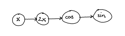
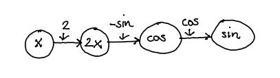
Suppose you want to compute the value of the function $h(x) = \sin(\cos(2 x))$ for $x = 0$ . Then you would start by evaluating the inner function $2 x$ , then applying $\cos$ and finally $\sin$ . This computation can be illustrated in the (computational) graph

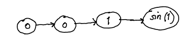
where you plug $x = 0$ into the leftmost node and fill in each node taking input from its left neighbor

Suppose we want to compute $h'(x)$ for $x = 0$ . Can we use the computational graph for this?

Recall the chain rule for functions of one variable. Here we have functions $f:(a, b)\rightarrow \RR$ and $g:(c, d)\rightarrow \RR$ , such that $g(x)\in (a, b)$ for $x\in (c, d)$ . If $g$ is differentiable at $x_0\in (c, d)$ and $f$ is differentiable at $g(x_0)\in (a, b)$ , the chain rule says that $f\circ g$ is differentiable at $x_0$ with

$(f\circ g)'(x_0) = f'(g(x_0)) g'(x_0).$

The chain rule tells us that

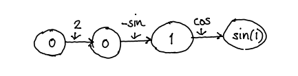
$h'(x) = \cos(\cos(2 x)) (- \sin( 2 x)) 2.$ This expression involves three derivatives corresponding to the three edges in the computational graph. We can illustrate the chain rule by labeling each edge with the derivative of its end node:

Then the derivative $h'(0)$ can be computed by as the product of the labels evaluated on their left nodes in the filled in computational graph:

i.e., $h'(0) = \cos(1) (-\sin(0)) 2$ . This observation is the basis of the famous backpropagation rule used in training neural networks.

The chain rule for functions of one variable generalizes verbatim to functions of several variables:

$(f\circ g)'(x_0) = f'( g(x_0)) g'(x_0)$ for compatible multivariate functions $f$ and $g$ when you replace usual multiplication by matrix multiplication.

Let $f:U\rightarrow \RR^m$ and $g: V\rightarrow \RR^d$ with $U\subseteq \RR^d$ , $V\subseteq \RR^l$ open subsets and $g(V)\subseteq U$ . If $g$ is differentiable at $v_0\in V$ and $f$ is differentiable at $g(v_0)\in U$ , then $f\circ g$ is differentiable at $v_0$ with

$(f\circ g)'(v_0) = f'( g(v_0)) g'(v_0). \tag{7.14}$

The proof of the chain rule in this general setting uses Definition 7.3 just as in the one variable case. It is not conceptually difficult, but severely cumbersome. We will not give it here.

7.7.1 Matrix multiplication graphically

To really understand the chain rule, it pays to view the matrix multiplication in (7.14) in a new light (inspired by computer science and neural networks).

An $m\times n$ matrix $(a_{ij})$ is a rectangular table with $m$ rows and $n$ columns containing $m n$ numbers. We may also view it as a (bipartite) graph with $m$ left nodes, $n$ right nodes and an edge from the left node $i$ to the right node $j$ with weight $a_{ij}$ . This is best illustrated by an example, which also tells you how matrix multiplication is (beautifully) interpreted in this setting.

The $2\times 3$ matrix

$A = \begin{pmatrix} 1 & 2 & 3\\ 4 & 5 & 6 \end{pmatrix}$ is represented below as a graph

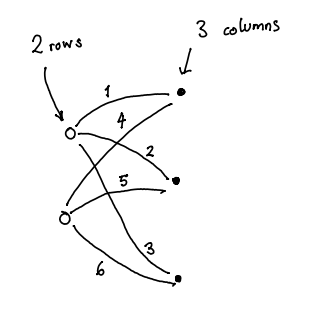
Similarly the $3\times 1$ matrix

$B = \begin{pmatrix} 7 \\ 8 \\ 9 \end{pmatrix}$ is represented as

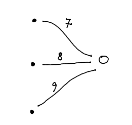
You know that the matrix product $A B$ is a $2\times 1$ matrix. Let us line $A$ and $B$ up graphically:

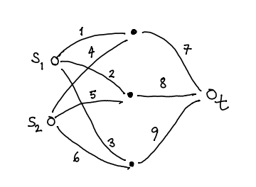
There are three paths from $s_1$ to $t$ and three paths from $s_2$ to $t$ . Here are the three paths from $s_1$ to $t$ :

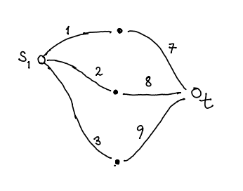
Finally, the matrix product $A B$ is represented by the graph

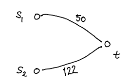
The number $50$ on the edge from $s_1$ to $t$ is gotten by adding the products of the weights on each of the three paths from $s_1$ to $t$ i.e., $1\cdot 7 + 2\cdot 8 + 3\cdot 9$ . This is the graphical interpretation of matrix multiplication!

7.7.2 Unpacking the chain rule

The matrix multiplication in (7.14) looks deceivingly simple. Let us write it out. Assume for simplicity that $g: \RR^l \rightarrow \RR^n$ is a function in the variables $x_1, \dots, x_l$ and that $f: \RR^n \rightarrow \RR^m$ is a function in the variables $y_1, \dots, y_n$ :

$g(x_1, \dots, x_l ) = \begin{pmatrix} g_1(x_1, \dots, x_l) \\ \vdots \\ g_n(x_1, \dots, x_l) \end{pmatrix} \qquad\text{and}\qquad f(y_1, \dots, y_n) = \begin{pmatrix} f_1(y_1, \dots, y_n) \\ \vdots \\ f_m(y_1, \dots, y_n) \end{pmatrix}.$ Then $h = (f\circ g):\RR^l\rightarrow \RR^m$ is a function in the variables $x_1, \dots, x_l$ :

$h(x_1, \dots, x_l) = \begin{pmatrix} h_1(x_1, \dots, x_l) \\ \vdots \\ h_m(x_1, \dots, x_l) \end{pmatrix}$ and we wish to compute $h'(v_0)$ , which is an $m\times l$ matrix with entries

$\pd{h_i}{x_j}(v_0),$ where $i = 1, \dots, m$ represent the rows and $j = 1, \dots, l$ the columns. Here (7.14) says that

$\pd{h_i}{x_j}(v_0) = \pd{f_i}{y_1}(g(v_0)) \pd{g_1}{x_j}(v_0) + \cdots + \pd{f_i}{y_n}(g(v_0)) \pd{g_n}{x_j}(v_0).$

When using the chain rule in computations it pays to use the graphical interpretation of matrix multiplication in subsection 7.7.1 with edges labeled by the derivatives in a computational graph. We illustrate this below.

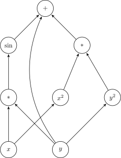
The function $h:\RR^2\rightarrow \RR$ given by

$h(x, y) = \frac{x^2+y}{x + \sin(x y)}$ may be evaluated using the computational graph

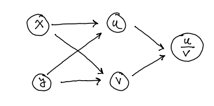
where $u$ is the function $u(x, y) = x^2+y$ and $v$ is the function $v(x, y) = x + \sin(x y)$ . Similar to the one variable case discussed in the beginning of section 7.7 , we label each edge, but now by the partial derivative of the function in its ending node with respect to the variable in its beginning node:

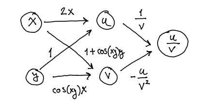
From the graphical interpretation of the matrix product and the chain rule you follow the two paths from the input node $x$ to the output node $u/v$ and conclude that

$\pd{h}{x} = \frac{2 x}{x + \sin(x y)} - \frac{x^2+y}{(x + \sin(x y))^2} (1 + \cos(x y) y).$

Here is another example of the chain rule in action through a computational graph. In the end you will see an implementation in a famous python library.

Consider the example

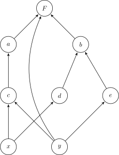
$f(x, y) = \sin(x y) + x^2 y^2 + y$ from Example 7.7 . Even though $f(x, y)$ superficially looks rather simple, it is composed of several smaller functions as displayed in the computational graph

Every node in the above graph, except the input nodes (with no ingoing arrows), represents some function $f:\RR^d\rightarrow \RR^m$ . For example the node $\sin$ represents a function $f: \RR\rightarrow \RR$ and $*$ represents a function $f: \RR^2\rightarrow \RR$ .

To emphasize that the non-input nodes really are functions we replace them by letters:

Here we see that

$f(x, y) = F(a(c(x, y)), y, b(d(x), e(y))),$ where

$\begin{aligned} F(a, y, b) &= a + y + b\\ a(c) &= \sin(c)\\ c(x, y) &= x y\\ b(d, e) &= d e\\ d(x) &= x^2\\ e(y) &= y^2 \end{aligned}$

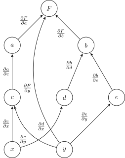
The gradient is then available from the decorated graph below

by multiplying the decorations on each path from the top to the input variable and the summing up. For example,

$\pd{F}{x} = \pd{F}{a} \pd{a}{c} \pd{c}{x} + \pd{F}{b} \pd{b}{d} \pd{d}{x}.$

Computational graphs and the chain rule are important components in machine learning libraries. Below is an example of the computation of $\pd{F}{x}$ in the computational graph above using the sympy library.

Live Python

7.7.3 Backpropagation from scratch

There is no magic in how sympy — or pytorch — computes these derivatives. The complete mechanism is the recipe you just used by hand: label every edge of the computational graph with the derivative of its end node with respect to its beginning node, multiply the labels along each path from the output down to an input, and add up the products. The program below implements exactly this and nothing more, in about twenty five lines.

A Node holds a number together with the edges of the computational graph: which nodes it was computed from, and the label on each incoming edge. Each operation writes down its own edge labels — for instance $d(u v)/du = v$ for a product. The function backprop then walks every path backwards from the output, multiplying the labels as it goes and adding the product into grad when it reaches a node.

Live Python

from math import sin, cos

class Node:
    """A number in a computational graph. It remembers the nodes it
    was computed from and the derivative along each incoming edge."""
    def __init__(self, value, edges=()):
        self.value = value
        self.edges = edges   # pairs: (parent node, edge label)
        self.grad = 0

def __add__(self, other):
        # edge labels: d(u + v)/du = 1  and  d(u + v)/dv = 1
        return Node(self.value + other.value, [(self, 1), (other, 1)])

def __mul__(self, other):
        # edge labels: d(u * v)/du = v  and  d(u * v)/dv = u
        return Node(self.value * other.value,
                    [(self, other.value), (other, self.value)])

def sine(u):
    # edge label: d sin(u)/du = cos(u)
    return Node(sin(u.value), [(u, cos(u.value))])

def backprop(node, path_product=1):
    # multiply the labels along every path from the output node,
    # and add up the products arriving at each node
    node.grad += path_product
    for parent, label in node.edges:
        backprop(parent, path_product * label)

# the computational graph of F = sin(x y) + x^2 y^2 + y  at (1, 1)
x = Node(1.0)
y = Node(1.0)

c = x * y
d = x * x
e = y * y
b = d * e
a = sine(c)
F = a + b + y

print("F(1, 1) =", F.value)
backprop(F)
print("dF/dx =", x.grad)   # sympy said: cos(1) + 2 = 2.5403...
print("dF/dy =", y.grad)

Compare with the sympy window above: the same numbers come out. Two details are worth savoring. First, $d = x \cdot x$ records two edges into $x$ , each with label $x$ — so the two paths contribute $x + x = 2x$ , and the power rule appears all by itself. Second, backprop is the graphical matrix multiplication of subsection 7.7.1 in executable form: every path is followed, the labels along it are multiplied, and parallel paths are added.

When you train neural networks in Section 7.9 , the backward pass is this walk written out with matrices. And pytorch's celebrated autograd is again this walk, organized so that each node is visited only once (in reverse order of computation), which is what lets it scale to graphs with billions of nodes.

Construct a computational graph for

$f(x, y) = x^3 + x y + y^3$ and detail the computation of the gradient $\nabla f$ in this context.

Compute the gradient of $f$ at $(x, y) = (1, 1)$ using the sympy window above (or pytorch in Google Colab).

Consider $f: \RR\rightarrow \RR^3$ and $g:\RR^3\rightarrow \RR$ given by

$f(t) = \begin{pmatrix} t\\ t^2\\ t^3 \end{pmatrix}\qquad \text{and}\qquad g \begin{pmatrix} x\\ y\\ z \end{pmatrix} = x^2 + 3 y^6 + 2 z^5.$ Compute $(g\circ f)'(t)$ using the chain rule and check the result with an explicit computation of the derivative of $g\circ f: \RR\rightarrow \RR$ .

We wish to show that the function $f: \RR^2 \rightarrow \RR$ given by

$f(x, y) = x^2 + y^2$ is convex. This means that we need to prove that

$f((1-t)x_0 + t x_1, (1-t) y_0 + t y_1) \leq (1-t) f(x_0, y_0) + t f(x_1, y_1)$ for every $(x_0. y_0), (x_1, y_1)\in \RR^2$ and every $t$ with $0\leq t\leq 1$ . This can be accomplished from the one variable case in the following way. Define

$g(t) = f((1-t)x_0 + t x_1, (1-t) y_0 + t y_1)$ and show that $g$ is convex by using the chain rule to show that $g''(t) \geq 0$ . Show how the convexity of $f$ follows from this by using that

$g(t) = g((1-t)\cdot 0 + t\cdot 1).$

7.8 Logistic regression

The beauty of the sigmoid function is that it takes any value $x\in \RR$ and turns it into a probability $0< \sigma(x) < 1$ by

$\sigma(x) = \frac{1}{1 + e^{-x}},$ i.e., $\sigma(-\infty) = 0$ and $\sigma(\infty) = 1$ .

Graph of the sigmoid function

Live Python

Prove that

$\sigma'(x) = \sigma(x) (1-\sigma(x))$ and

$\log \frac{\sigma(x)}{1-\sigma(x)} = x.$

We will not go into all the details (some of which can be traced to introductory probability and statistics), but suppose that we have an outcome $E$ , which may or may not happen.

We have an idea, that the probability of $E$ is dependent on certain parameters $w_0, w_1, \dots, w_n$ and observations $x_1, \dots, x_n$ that fit into the sigmoid function as

$p(x_1, \dots, x_n) = \sigma(w_0 + w_1 x_1 + \cdots + w_n x_n) = \frac{1}{1 + e^{-w_0 - w_1 x_1 - \cdots - w_n x_n}}. \tag{7.15}$

An example of this could be where $x_1, \dots, x_{784}$ denote the gray scale of each pixel in a $28\times 28$ image. The event $E$ is whether the image contains the digit $4$ :

Here $p(x_1, \dots, x_{784})$ would be the probability that the image contains the digit $4$ .

7.8.1 Estimating the parameters

Suppose also that we have a table of observations (data set)

$\begin{matrix} x_{11} & \cdots & x_{1n} & E_1\\ x_{21} & \cdots & x_{2n} & E_2\\ \vdots & \ddots & \vdots & \vdots\\ x_{m1} & \cdots & x_{mn} & E_m, \end{matrix} \tag{7.16}$

where each row has observations $x_{i1}, \dots, x_{in}$ along with a binary variable $E_i$ , which is $1$ if $E$ was observed to occur and $0$ if not.

Assuming that (7.15) holds, the probability of observing the $m$ observations in (7.16) is

$\prod_{i=1}^m p(x_{i1}, \dots, x_{in})^{E_i} (1 - p(x_{i1}, \dots, x_{in}))^{1-E_i}. \tag{7.17}$ Notice that (7.17) is a function $L(w_0, \dots, w_n)$ of the parameters $w_0, w_1, \dots, w_n$ for fixed observations $x_{ij}$ .

We wish to choose the parameters so that $L(w_0, w_1, \dots, w_n)$ is maximized (this is called maximum likelihood estimation). So we are in fact here, dealing with an optimization problem, which is usually solved by gradient descent (for $-L$ ) or solving the equations

$\nabla L (w_0, w_1, \dots, w_n) = 0.$

Instead of maximizing $L(w_0, \dots, w_n)$ one usually maximizes the logarithm

$\begin{aligned} \ell(w_0, w_1, \dots, w_n) &= \log L(w_0, w_1, \dots, w_n)\\ &= \sum_{i=1}^m E_i \log p(x_{i1}, \dots, x_{in}) + (1 - E_i) \log ( 1 - p(x_{i1}, \dots, x_{in}))\\ &= \sum_{i=1}^m E_i (w_0 + w_1 x_{i1} + \cdots + w_n x_{in}) - \log (1 + e^{w_0 + w_1 x_{i1} + \cdots + w_n x_{in}}). \end{aligned}$

Notice that we have used Exercise 7.30 and the logarithm rules $\log(a b) = \log(a) + \log(b)$ and $\log(a/b) = \log(a) - \log(b)$ in the computation above.

Suppose that the event $E$ is assumed to be dependent on only one observation $x$ i.e., $n=1$ above. For example, $E$ could be the event of not showing up on a Monday paired with the amount of sleep $x$ in the weekend.

Here

$p(x) = \sigma(\alpha + \beta x)$ and

$\begin{aligned} \ell(\alpha, \beta) &= \sum_{i=1}^m E_i \log p(x_i) + (1 - E_i)\log (1-p(x_i))\\ &= \sum_{i=1}^m E_i (\alpha + \beta x_i) - \log(1 + e^{\alpha + \beta x_i}). \end{aligned}$

Explain how the end result of the computation of $\ell(\alpha, \beta)$ in Example 7.31 is obtained and compute $\nabla \ell (\alpha, \beta)$ .

I remember exactly where I was when first hearing about the Challenger ² See byuistats.github.io for more details on this example disaster in 1986.

This dreadful event was caused by failure of a socalled O-ring. The O-rings had been tested before the launch for failure (=1 below) at different temperatures (in F) resulting in the (partial) table below.

$\begin{matrix} 53.0 & 1\\ 56.0 & 1\\ 57.0 & 1\\ 63.0 & 0\\ \vdots & \vdots\\ 70.0 & 0\\ 70.0 & 1\\ \vdots & \vdots\\ 79.0 & 0 \end{matrix}$ At the morning of the launch the outside temperature was (uncharacteristically low for Florida) $31$ degrees Fahrenheit. We wish to use logistic regression to compute the probability that the O-ring fails.

The model $p(x) = \sigma(\alpha + \beta x)$ is exactly a single neuron — the one you will train again in Section 7.9 — and we can fit it right here with the tools of this chapter, no library and no black box: maximize $\ell(\alpha, \beta)$ from Example 7.31 by gradient ascent, i.e., repeat

$(\alpha, \beta) := (\alpha, \beta) + \lambda\, \nabla \ell(\alpha, \beta).$ We walk with the gradient, since we are maximizing.

One preparation first — a step used everywhere in machine learning. We standardize the input:

$z = \frac{x - \bar{x}}{s},$ where

$\bar{x} = \frac{x_1 + \cdots + x_m}{m} \qquad\text{and}\qquad s^2 = \frac{(x_1 - \bar{x})^2 + \cdots + (x_m - \bar{x})^2}{m}$ are the mean and the variance of the $m = 24$ temperatures ( $s$ is the standard deviation). The standardized inputs $z$ have mean $0$ and standard deviation $1$ — small, comparable numbers around $0$ , no matter how the raw data are scaled. Why we bother will become clear in a moment, when we try skipping this step. We train the neuron $\sigma(a + b z)$ on the standardized input and translate back afterwards. Nothing is lost in the translation, because

$a + b z = a + b\, \frac{x - \bar{x}}{s} = \left(a - \frac{b\, \bar{x}}{s}\right) + \frac{b}{s}\, x,$ so the trained neuron $\sigma(a + b z)$ is the same function of the original temperature $x$ as $\sigma(\alpha + \beta x)$ with

$\beta = \frac{b}{s} \qquad\text{and}\qquad \alpha = a - \frac{b\, \bar{x}}{s}.$

Live Python

import numpy as np
import matplotlib.pyplot as plt

# temperature (F) and O-ring failure (1) or not (0)
x = np.array([53, 56, 57, 63, 66, 67, 67, 67, 68, 69, 70, 70,
              70, 70, 72, 73, 75, 75, 76, 76, 78, 79, 80, 81], dtype=float)
E = np.array([1, 1, 1, 0, 0, 0, 0, 0, 0, 0, 0, 1,
              0, 1, 0, 0, 0, 1, 0, 0, 0, 0, 0, 0], dtype=float)

def sigmoid(t):
    return 1/(1 + np.exp(-t))

xbar, s = x.mean(), x.std()   # standardize the input ...
z = (x - xbar)/s

a, b = 0.0, 0.0               # ... and train the neuron sigmoid(a + b z)
lam = 0.1
for step in range(2000):
    p = sigmoid(a + b*z)              # the neuron's predictions
    a += lam*(E - p).sum()            # gradient ASCENT on l(a, b):
    b += lam*((E - p)*z).sum()        # these two lines are grad l

alpha = a - b*xbar/s                  # translate back to
beta = b/s                            # p = sigmoid(alpha + beta x)
print(f"alpha = {alpha:.4f},  beta = {beta:.4f}")
print("Probability of failure at 31 degrees Fahrenheit =",
      round(sigmoid(alpha + beta*31), 4))

t = np.linspace(25, 85, 300)
plt.plot(t, sigmoid(alpha + beta*t))
plt.plot(x, E, "ko")
plt.axvline(31, color="red", linestyle="--")
plt.xlabel("temperature (F)")
plt.ylabel("probability of O-ring failure")
plt.grid(True)
plt.show()

The mathematics was there before the launch: at $31$ degrees Fahrenheit the trained neuron puts the probability of O-ring failure at $0.997$ .

So why did we standardize? Try the ascent directly on the raw temperatures and watch it fail, miserably — seeing how it fails teaches more than the success did. The cell below tries: $2000$ steps with $\lambda = 0.1$ , starting from $(\alpha, \beta) = (0, 0)$ . The two gradient lines in the loop are precisely $\nabla \ell$ from the exercise above — the only change from the successful cell is the missing standardization.

Live Python

At a maximum the gradient is $(0, 0)$ . The cell reports the gradient $(6, 381)$ — after $2000$ steps the ascent is nowhere near the top. The culprit is the factor $x_i \approx 70$ in the second coordinate of the gradient. The very first step is

$\beta := 0 + 0.1 \sum_{i=1}^{24} \left(E_i - \tfrac{1}{2}\right) x_i \approx -45.8,$ which makes $\alpha + \beta x_i \approx -3200$ . Then $e^{3200}$ overflows, every probability $p(x_i)$ snaps to $0$ or $1$ , and from there the ascent bounces back and forth without ever settling down. Shrinking the learning rate does not save us: with $\lambda = 0.00001$ the $\beta$ -updates calm down, but now $\alpha$ — which has to climb above $11$ — moves in steps of size about $10^{-5}$ . Rerun the cell with this $\lambda$ and watch $\alpha$ barely leave $0$ ; even two million steps would only push it to about $0.9$ . One fixed learning rate cannot serve two parameters living on such different scales — standardization put them on the same scale, and the ascent sailed home.

Professional libraries fit logistic regression in a few lines. Run the scikit-learn code below and compare $\alpha$ , $\beta$ and the failure probability with the neuron trained in Example 7.33 .

Live Python

The option solver='lbfgs' chooses an algorithm for maximizing $\ell(\alpha, \beta)$ and C=25 controls a socalled regularization. Try removing C=25 first and then solver='lbfgs'. What happens?

Chatbot Prompt

Explain the function LogisticRegression in sklearn. In particular, what do the parameters in

model = LogisticRegression(C=25, solver='lbfgs') model.fit(X,y)

mean?

In the button below is a naive implementation of gradient ascent for the Challenger data set — a variant of the training in Example 7.33 that adjusts the step size with successive negative powers of $2$ , as in the introduction to this chapter, instead of standardizing the input. Run experiments with different initial values and number of iterations, and compare the quality of the solutions in terms of the gradient (which is available in the output from the Naive code).

Yes, you are allowed (and encouraged) to use generative AI tools here!

Naive code

Live Python

import numpy as np

x0 = [1, 1]
noofits = 20

x = np.array([53.0, 56.0, 57.0, 63.0, 66.0, 67.0, 67.0, 67.0,
              68.0, 69.0, 70.0, 70.0, 70.0, 70.0, 72.0, 73.0,
              75.0, 75.0, 76.0, 76.0, 78.0, 79.0, 80.0, 81.0])
E = np.array([1.0, 1.0, 1.0, 0.0, 0.0, 0.0, 0.0, 0.0,
              0.0, 0.0, 0.0, 1.0, 0.0, 1.0, 0.0, 0.0,
              0.0, 1.0, 0.0, 0.0, 0.0, 0.0, 0.0, 0.0])

Es = E.sum()
Exs = (x*E).sum()

def sigmoid(a, b, t):
    return 1/(1 + np.exp(-a - b*t))

def ell(v):
    a, b = v
    return (E*(a + b*x) - np.log(1 + np.exp(a + b*x))).sum()

def gradient(v):
    a, b = v
    return np.array([Es - sigmoid(a, b, x).sum(),
                     Exs - (x*sigmoid(a, b, x)).sum()])

def gradientascent(v0):
    l0 = ell(v0)
    d = gradient(v0)
    k = 0
    while True:
        v1 = v0 + 2.0**(-k)*d
        if ell(v1) > l0:
            break
        k += 1
    return v1

v = np.array(x0, dtype=float)
for k in range(noofits):
    v = gradientascent(v)

print("x0 = ", x0)
print("Number of gradient ascents (maximization problem) =  ", noofits)
print("Predicted maximal point =  ", v)

alpha, beta = v

print("Gradient at predicted maximal point = ", gradient(v))
print("Predicted probability of failure at 31F = ", sigmoid(alpha, beta, 31))

7.9 Training neural networks

Every ingredient is now on the table: partial derivatives, the gradient, the chain rule on computational graphs, gradient descent (Section 7.5.1 ) and the activation functions — sigmoid and ReLU — from the very first chapter. In this section we put them to work and train genuine neural networks — first one so small that every number can be inspected by hand, then one that reads handwritten digits, and in the end one that writes. Everything runs live in these notes, and no mathematics beyond this chapter is involved.

7.9.1 A single neuron

The smallest neural network is a single neuron with one input: it takes a number $x$ , forms $b + w x$ and applies the sigmoid function,

$y = \sigma(b + w x) = \frac{1}{1 + e^{-b - w x}}.$ The numbers $w$ and $b$ are called the weight and the bias. They are the parameters the network is allowed to change when it learns. You have seen this function before: it is exactly the probability (7.15) of logistic regression — a single neuron is logistic regression.

Run the cell below to see how $w$ and $b$ bend and shift the sigmoid, then change the values and rerun.

Live Python

7.9.2 Training a single neuron

Training means: choose $w$ and $b$ so that the neuron reproduces known data as well as possible. Suppose eight students report how many hours $x_i$ they studied and whether they passed ( $E_i = 1$ ) or failed ( $E_i = 0$ ) an exam. (You met these eight students in Exercise 5.22 , where the best straight line through the data predicted "probabilities" beyond $1$ — here comes the better idea it promised.) A neuron with sigmoid activation is the logistic model of Section 7.8 , so we already know what "as well as possible" should mean: maximize the log-likelihood. Machine learning prefers to minimize, so we flip the sign and call the result the cross-entropy loss: writing $y_i = \sigma(b + w x_i)$ ,

$L(w, b) = -\sum_{i=1}^8 \Bigl( E_i \ln y_i + (1 - E_i)\ln(1 - y_i)\Bigr),$ which we minimize by gradient descent — the same computation as gradient ascent on $\ell$ , in new clothes. The gradient is a small miracle of cancellation. By the chain rule and the formula $\sigma'(z) = \sigma(z)(1 - \sigma(z))$ from Exercise 7.30 , the $i$ -th term of $L$ responds to the sum $z_i = b + w x_i$ at the rate

$-\left(\frac{E_i}{y_i} - \frac{1 - E_i}{1 - y_i}\right) y_i (1 - y_i) = y_i - E_i$ — the derivative of the sigmoid cancels completely, leaving

$\pd{L}{w} = \sum_{i=1}^8 (y_i - E_i)\, x_i \qquad\text{and}\qquad \pd{L}{b} = \sum_{i=1}^8 (y_i - E_i).$ Prediction too high: push down. Prediction too low: push up. Every data point pushes with a force equal to its error — few formulas in machine learning are used more often than this one. It is all a neural network library ever does, just for many more parameters. The training loop below is four lines.

Live Python

import numpy as np
import matplotlib.pyplot as plt

# hours of study, and exam passed (1) or failed (0)
x = np.array([0.5, 1.0, 1.5, 2.0, 3.0, 4.0, 5.0, 6.0])
E = np.array([0,   0,   0,   0,   1,   1,   1,   1  ])

def sigmoid(z):
    return 1/(1 + np.exp(-z))

w, b = 0.0, 0.0     # start knowing nothing
lam = 0.1           # learning rate (found by experiment, as always)

losses = []
for step in range(3000):
    y = sigmoid(b + w*x)                       # the neuron's predictions
    losses.append(-(E*np.log(y) + (1 - E)*np.log(1 - y)).sum())
    dw = ((y - E)*x).sum()      # dL/dw: each point pushes by its error
    db = (y - E).sum()          # dL/db
    w -= lam*dw
    b -= lam*db

print(f"learned w = {w:.2f}, b = {b:.2f}")
print("P(pass | 2.5 hours of study) =", round(sigmoid(b + w*2.5), 3))

fig, (ax1, ax2) = plt.subplots(1, 2, figsize=(9, 3.5))
xs = np.linspace(0, 7, 200)
ax1.scatter(x, E, color="red", zorder=3)
ax1.plot(xs, sigmoid(b + w*xs))
ax1.set_title("the trained neuron")
ax1.grid(True)
ax2.plot(losses)
ax2.set_title("loss during training")
ax2.grid(True)
plt.show()

The right hand plot is the famous loss curve — the first thing every machine learning engineer looks at during training. The left hand plot shows what the neuron has learned: a threshold around $2.5$ hours of study. One thing to notice: because the data are perfectly separated at $2.5$ hours, longer training keeps steepening the threshold — the weights grow forever, chasing probabilities $0$ and $1$ they can never quite reach. Real data are rarely this clean. Play with the data and watch the neuron adapt.

7.9.3 A genuine network: solving XOR

A single neuron has a hard limit. In Exercise 5.9 you showed that no line separates the four points $(0,0), (1,1)$ (labeled blue) and $(0,1), (1,0)$ (labeled red) — and a single neuron can only draw a line. This little data set, known as XOR, famously stalled neural network research for years.

The way out is to compose neurons into a network with a hidden layer: two neurons look at the input, and a third neuron looks at what they found,

$\begin{aligned} h_1 &= \sigma(b_1 + w_{11} x_1 + w_{21} x_2)\\ h_2 &= \sigma(b_2 + w_{12} x_1 + w_{22} x_2)\\ y &= \sigma(c + v_1 h_1 + v_2 h_2). \end{aligned}$ The composed function is no longer a bent line — and thanks to the chain rule we can still compute the gradient of the cross-entropy loss with respect to all nine parameters; the miraculous $y - E$ cancellation from the single neuron applies to the output neuron unchanged. The code below does exactly that in vectorized form: the forward pass evaluates the network, the backward pass walks the computational graph in reverse, exactly as in Section 7.7 . This is backpropagation.

Live Python

import numpy as np
import matplotlib.pyplot as plt

X = np.array([[0, 0], [0, 1], [1, 0], [1, 1]], dtype=float)
t = np.array([0, 1, 1, 0], dtype=float)    # the XOR labels

def sigmoid(z):
    return 1/(1 + np.exp(-z))

rng = np.random.default_rng(1)
W1 = rng.normal(0, 1, (2, 2))   # weights: input -> hidden
b1 = np.zeros(2)                # biases of the two hidden neurons
W2 = rng.normal(0, 1, 2)        # weights: hidden -> output
b2 = 0.0

lam = 1.0                       # learning rate
for step in range(4000):
    # forward pass: evaluate the network
    h = sigmoid(X @ W1 + b1)
    y = sigmoid(h @ W2 + b2)
    # backward pass: the chain rule, edge by edge
    dy  = y - t                 # the cross-entropy gradient again
    dW2 = h.T @ dy
    db2 = dy.sum()
    dh  = np.outer(dy, W2) * h*(1 - h)
    dW1 = X.T @ dh
    db1 = dh.sum(axis=0)
    # the gradient descent step
    W1 -= lam*dW1; b1 -= lam*db1
    W2 -= lam*dW2; b2 -= lam*db2

print("network outputs:", np.round(y, 3))
print("XOR labels:     ", t)

# color the plane by the network's output
g1, g2 = np.meshgrid(np.linspace(-0.5, 1.5, 200), np.linspace(-0.5, 1.5, 200))
grid = np.column_stack([g1.ravel(), g2.ravel()])
z = sigmoid(sigmoid(grid @ W1 + b1) @ W2 + b2).reshape(g1.shape)

plt.contourf(g1, g2, z, levels=20, cmap="coolwarm")
plt.colorbar()
plt.scatter([0, 1], [0, 1], color="blue", s=60, edgecolor="black")
plt.scatter([0, 1], [1, 0], color="red", s=60, edgecolor="black")
plt.title("what the network computes")
plt.show()

Look at the picture: the network has invented a diagonal band — a shape no single line can produce. Each hidden neuron contributes one line, and the output neuron combines them. Deep learning is this phenomenon repeated at scale.

Backpropagation by hand. Consider the simple chain network

where

$\begin{aligned} z_2 = \sigma_1(z_1) = \sigma(a + b z_1)\\ z_3 = \sigma_2(z_2) = \sigma(c + d z_2)\\ z_4 = \sigma_3(z_3) = \sigma(e + f z_3), \end{aligned}$ and $\sigma$ is the sigmoid function. This neural network has input $z_1$ and output $z_4$ . Let $C$ be a function of the output $z_4$ . For fixed $z_1$ , we consider $C$ as a function of $a, b, c, d, e, f$ via

$F\begin{pmatrix} a\\ b\\ c\\ d\\ e\\ f\end{pmatrix} = C(\sigma_3(\sigma_2(\sigma_1(z_1)))).$ Backpropagation for training neural networks is using the chain rule for computing the gradient

$\nabla F = \left( \pd{F}{a}, \pd{F}{b}, \pd{F}{c}, \pd{F}{d}, \pd{F}{e}, \pd{F}{f} \right).$ Explain how to do this — it is exactly what the backward pass in the code above does.

7.9.4 Reading handwritten digits

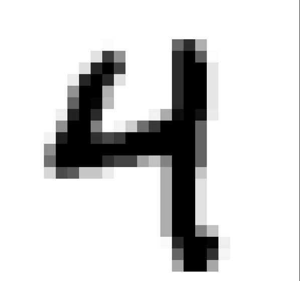
We end with real data: images of handwritten digits. The sklearn library ships $1797$ small $8\times 8$ gray scale images. Before training anything, look at the data — the cell below shows the first image in the collection together with the $8\times 8$ matrix of gray values behind it.

Live Python

An image is nothing but an $8\times 8$ matrix of numbers. Flattening the matrix row by row turns it into a vector in $\RR^{64}$ — and the machinery of this chapter applies. The network we now train is a composition

$\RR^{64} \longrightarrow \RR^{32} \longrightarrow \RR^{10},$ exactly as promised in the very first chapter. Written out: an image, stored as a row vector $x\in \RR^{64}$ , is processed in two layers

$\begin{aligned} h &= \operatorname{act}(x\, W_1 + b_1)\\ y &= \sigma(h\, W_2 + b_2), \end{aligned}$ where $W_1$ is a $64\times 32$ matrix of weights, $b_1\in \RR^{32}$ holds the biases of the $32$ hidden neurons, $W_2$ is a $32\times 10$ matrix and $b_2\in \RR^{10}$ . Output number $d$ of $y\in \RR^{10}$ is a score between $0$ and $1$ for "this image shows the digit $d$ " — ten separate yes/no neurons, so the scores need not sum to $1$ — and the network's guess is the output with the largest score. Counting as in the first chapter, the network has

$64\cdot 32 + 32 + 32\cdot 10 + 10 = 2410$ parameters — all of them trained by gradient descent, in your browser.

The hidden activation function $\operatorname{act}$ is your choice in the code: the sigmoid or the ReLU from the first chapter. The output layer always uses the sigmoid, so that its ten scores land between $0$ and $1$ . Backpropagation only needs the derivative of the activation: $\sigma'(z) = \sigma(z)(1 - \sigma(z))$ for the sigmoid, while the ReLU has derivative $1$ for $z > 0$ and $0$ for $z < 0$ — this is the function dact in the code.

Before you run it, read the code with this dictionary. The $1500$ training images are stacked as the rows of the matrix Xtr, so Xtr @ W1 + b1 computes all $1500$ hidden vectors in one matrix multiplication. The line T = np.eye(10)[labels] turns the digit $d$ into the target vector with $1$ in entry $d$ and $0$ elsewhere (one-hot encoding — the same trick as for words in Chapter 5). The loss is the cross-entropy, summed over the ten outputs — exactly as for the single neuron, ten times.

So how does the code find all $2410$ partial derivatives? This is backpropagation, and it is nothing but the chain rule of Section 7.7 — the nudge bookkeeping of Section 7.6 — organized cleverly. Let us walk through it for a single image $x$ with target vector $t$ . Write the two layers with their intermediate sums,

$\begin{aligned} z^{(1)} &= x\, W_1 + b_1, & h &= \operatorname{act}(z^{(1)}),\\ z^{(2)} &= h\, W_2 + b_2, & y &= \sigma(z^{(2)}), \end{aligned}$ and let

$L = -\sum_{d=1}^{10} \Bigl( t_d \ln y_d + (1 - t_d)\ln(1 - y_d)\Bigr)$ be the cross-entropy loss.

Start at the loss and move backwards. How much does $L$ respond to a nudge of the sum $z^{(2)}_d$ entering output neuron $d$ ? The nudge passes through the sigmoid and into the $d$ -th term of the loss — and the single-neuron cancellation strikes again:

$\delta^{(2)}_d = \pd{L}{z^{(2)}_d} = y_d - t_d.$ This is the line dy in the code. With $\delta^{(2)}$ in hand, the gradients of the output layer's parameters are immediate: the weight $(W_2)_{jd}$ enters the sum $z^{(2)}_d$ multiplied by $h_j$ , so

$\pd{L}{(W_2)_{jd}} = h_j\, \delta^{(2)}_d \qquad\text{and}\qquad \pd{L}{(b_2)_d} = \delta^{(2)}_d$ — the lines dW2 and db2.

Push the nudge one layer further back. The hidden value $h_j$ influences the loss through all ten outputs, one path per output neuron, so its exchange rate is a sum over the ten paths — exactly as in the computational graphs of Section 7.7.1 :

$\pd{L}{h_j} = \sum_{d=1}^{10} \delta^{(2)}_d\, (W_2)_{jd}.$ Passing the nudge through the activation of hidden neuron $j$ then gives

$\delta^{(1)}_j = \pd{L}{z^{(1)}_j} = \left(\sum_{d=1}^{10} \delta^{(2)}_d\, (W_2)_{jd}\right) \operatorname{act}'\bigl(z^{(1)}_j\bigr)$ — the line dh, where the sum over $d$ is the matrix product dy @ W2.T and $\operatorname{act}'$ is the function dact. The first layer's gradients now follow exactly as before:

$\pd{L}{(W_1)_{ij}} = x_i\, \delta^{(1)}_j \qquad\text{and}\qquad \pd{L}{(b_1)_j} = \delta^{(1)}_j$ — the lines dW1 and db1.

Notice the economy of the scheme. One forward pass stores $h$ and $y$ ; one backward pass computes $\delta^{(2)}$ and then $\delta^{(1)}$ ; and out come all $2410$ partial derivatives. The price of the whole gradient is roughly two evaluations of the network, no matter how many parameters there are — this is why the loss nudges are propagated backwards, layer by layer, and why the method is called backpropagation. Finally, the code does all of this for the $1500$ training images at once: stacking the images as rows turns the products $h_j\, \delta^{(2)}_d$ into the matrix product h.T @ dy, which sums over the images automatically, and the division by len(Xtr) makes $L$ the mean loss over the data. Training takes a few seconds.

Live Python

import numpy as np
import matplotlib.pyplot as plt
from sklearn.datasets import load_digits

digits = load_digits()
X = digits.data / 16.0          # 1797 images, flattened to vectors in R^64
labels = digits.target

T = np.eye(10)[labels]          # one-hot targets: row i has a 1 in entry labels[i]

Xtr, Xte = X[:1500], X[1500:]   # train on 1500 images ...
Ttr = T[:1500]
lte = labels[1500:]             # ... test on the remaining 297

activation = "sigmoid"          # your choice: "sigmoid" or "relu"

def sigmoid(z):
    return 1/(1 + np.exp(-z))

def act(z):
    return np.maximum(0, z) if activation == "relu" else sigmoid(z)

def dact(h):                    # derivative, in terms of h = act(z)
    return (h > 0)*1.0 if activation == "relu" else h*(1 - h)

rng = np.random.default_rng(0)                  # small random start: with all
W1 = rng.normal(0, 0.5, (64, 32)); b1 = np.zeros(32)   # weights equal, all
W2 = rng.normal(0, 0.5, (32, 10)); b2 = np.zeros(10)   # neurons would stay equal

lam = 0.5 if activation == "sigmoid" else 0.1   # relu needs smaller steps
for step in range(4000):
    h = act(Xtr @ W1 + b1)                      # hidden layer
    y = sigmoid(h @ W2 + b2)                    # output layer: ten scores
    dy  = (y - Ttr) / len(Xtr)                  # backward pass ...
    dW2 = h.T @ dy;   db2 = dy.sum(axis=0)
    dh  = dy @ W2.T * dact(h)                   # ... through act via dact
    dW1 = Xtr.T @ dh; db1 = dh.sum(axis=0)
    W1 -= lam*dW1; b1 -= lam*db1                # gradient descent
    W2 -= lam*dW2; b2 -= lam*db2

pred = np.argmax(sigmoid(act(Xte @ W1 + b1) @ W2 + b2), axis=1)
print("hidden activation:", activation)
print("accuracy on the 297 unseen images: %.1f%%" % (100*(pred == lte).mean()))

fig, axes = plt.subplots(1, 10, figsize=(10, 1.6))
for ax, i in zip(axes, range(10)):
    ax.imshow(digits.images[1500 + i], cmap="gray_r")
    ax.set_title(str(pred[i]), color="black" if pred[i] == lte[i] else "red")
    ax.axis("off")
plt.show()

Now switch activation to "relu" and rerun. Which activation reads more of the unseen images correctly here? Notice that the ReLU asks for a smaller learning rate — its unbounded output makes big steps dangerous.

Around nine out of ten unseen images are read correctly — by a network you trained from scratch and whose every line of mathematics you have now met. Scaling this recipe up is modern AI: more pixels, more layers, and libraries such as pytorch that apply the chain rule automatically to computational graphs with billions of nodes — exactly the graphs of Section 7.7 . Such libraries do not run inside a web page, but you can use them for free in Google Colab.

7.9.5 A network that writes

The networks above read: they take an image and answer a question about it. But the neural network you use every day — the chatbot from Section 1.1 — writes. That looks like a completely different ability. It is not. Writing is reading in disguise: a network writes by answering, over and over again, the classification question

$\text{"given the text so far, which symbol comes next?"}$ picking a symbol according to the answer, appending it to the text and asking again. In this final section you will train a genuine writing network. A chatbot learns from trillions of words; we scale the idea down to a miniature that learns from a couple of hundred Danish first names — and then invents new ones.

Here is the plan. Our alphabet consists of the letters that occur in the names plus a special symbol "." marking the end of a name — $27$ symbols in all. The network gets a context of $C = 3$ consecutive symbols and must predict the symbol that follows. Every name in the list becomes a handful of training examples; padding with dots supplies the start, and the final dot teaches the network how names end. The name anna alone contributes five:

$\text{"..."} \mapsto \text{"a"},\quad \text{"..a"} \mapsto \text{"n"},\quad \text{".an"} \mapsto \text{"n"},\quad \text{"ann"} \mapsto \text{"a"},\quad \text{"nna"} \mapsto \text{"."}$ Symbols become vectors by one-hot encoding, exactly as in (5.16) : each of the three context symbols becomes a one-hot vector in $\RR^{27}$ , and gluing the three together gives an input vector $x\in \RR^{81}$ . The target is one of $27$ classes. Structurally we are back at the digits network — reading handwritten digits was "which of $10$ classes?", writing names is "which of $27$ classes?", asked repeatedly.

One ingredient needs an upgrade. For writing, the $27$ output numbers must form a probability distribution: they must be positive and sum to $1$ , because we are going to roll a die weighted by them. The digits network used ten separate sigmoids, which obey no such constraint. The standard fix is the softmax function, which turns any vector $z\in\RR^V$ of scores into probabilities:

$\operatorname{softmax}(z)_j = \frac{e^{z_j}}{e^{z_1} + \cdots + e^{z_V}}. \tag{7.18}$ The exponentials make every output positive, and dividing by their sum makes the outputs sum to $1$ . You have met this recipe before: it is exactly (5.17) , which computed the attention weights in Section 5.5.3 — there the outputs weighted a blend of word vectors, here they are read as probabilities. Softmax is also the many-class face of the sigmoid (see Exercise 7.36 below).

As loss we keep cross-entropy in the form maximum likelihood handed us in (7.17) : if the correct next symbol has class $t$ and the network outputs the probabilities $y = \operatorname{softmax}(z)$ , the loss of the example is

$L = -\ln(y_t),$ the price for the probability the network gave to what actually came next. And now the small miracle of Section 7.9 repeats itself: the nudge of the loss with respect to the scores $z$ is again prediction minus target,

$\pd{L}{z_j} = y_j - t_j,$ where $t\in\RR^{27}$ is the one-hot target. This is the same formula that ran the single neuron, the XOR network and the digits network — so the backward pass below is, line for line, the code you have already studied.

Why the cancellation survives

Insert $y_t = e^{z_t}/(e^{z_1} + \cdots + e^{z_V})$ into the loss and use $\ln(a/b) = \ln(a) - \ln(b)$ :

$L = -\ln(y_t) = -z_t + \ln\left(e^{z_1} + \cdots + e^{z_V}\right).$ Now differentiate with respect to $z_j$ . The first term contributes $-1$ if $j = t$ and $0$ otherwise — that is exactly $-t_j$ . For the second term the chain rule gives

$\pd{}{z_j} \ln\left(e^{z_1} + \cdots + e^{z_V}\right) = \frac{e^{z_j}}{e^{z_1} + \cdots + e^{z_V}} = y_j,$ and adding the two contributions gives $\pd{L}{z_j} = y_j - t_j$ . Compare this with the computation for the single neuron in Section 7.9 — same cancellation, same reason: the derivative of $\ln$ undoes the exponential.

So the network is

$\RR^{81} \longrightarrow \RR^{64} \longrightarrow \RR^{27},$ a sigmoid hidden layer followed by a softmax output layer — counting as in Exercise 1.126 , that is $81\cdot 64 + 64 + 64\cdot 27 + 27 = 7003$ parameters. Before training these are small random numbers, so the network spreads its probability almost evenly over the $27$ symbols and the mean loss starts near $-\ln(1/27) = \ln(27) \approx 3.3$ : the loss of pure guessing. Watch it fall.

After training comes the payoff: writing. Start from the empty context "...", let the network output its $27$ probabilities, roll a die weighted by them, append the resulting symbol to the context and repeat — until the die shows ".": the network has decided that its name is finished. This is composition one last time: the network fed its own output, over and over. The cell below does all of it — the data, the training and twenty rolls of the die. Training takes a little longer than the digits network; the names are worth the wait.

Live Python

import numpy as np

# the entire universe this network will ever see: Danish first names
names = """
anders anna anne astrid aksel alberte alfred alma amalie andrea agnes arthur august aya
bertram bjørn bo brian birgitte bente bodil carl carla caroline cecilie charlotte christian
christina clara claus dagmar daniel david ditte dorthe ebbe edith eigil ejnar ella ellen
elias emil emilie emma erik erling esben ester eva felix filippa finn flemming freja frederik
frida frode gerda gitte gorm gustav hanne hans harald helle henrik herman hjalte holger
hugo ida inge ingrid isabella iver jakob jan jens jeppe jesper johan johanne jonas josefine
julie jørgen kaj karen karl karla kasper katrine kim kirsten kjeld klara klaus knud kristian
lars lasse laura lea leif lene liva lone lotte louise lukas mads magnus maja malou malthe
maren marie marius marcus mathilde merete mette mikkel mogens mona morten nanna niels
nikolaj nina noah nora oda olga oliver oscar osvald otto ove per pernille peter pia poul
preben rasmus rene rikke rolf rune sara selma signe sigrid silas simon sofia sofie solvej
sonja steen stine storm susanne svend søren tage thea theo thomas thorbjørn tina tobias
torben tove troels ulla ulrik valdemar vera vibeke victor viggo vilfred villads viola
william yrsa åse øjvind aage birthe carsten dorte elin erna gunnar gudrun hedvig
henning inger jytte kamma kurt lissy nanny orla ragnhild sigurd tordis valborg
""".split()

alphabet = sorted(set("".join(names))) + ["."]    # "." marks the end of a name
V = len(alphabet)
idx = {c: i for i, c in enumerate(alphabet)}
C = 3                                             # context: three symbols

xs, ts = [], []                                   # every name becomes training
for name in names:                                # pairs: "..." -> a, "..a" -> n,
    context = [idx["."]]*C                        # ".an" -> n, "ann" -> a,
    for ch in name + ".":                         # "nna" -> .
        xs.append(context.copy()); ts.append(idx[ch])
        context = context[1:] + [idx[ch]]
xs, ts = np.array(xs), np.array(ts)
X = np.eye(V)[xs].reshape(len(xs), C*V)           # one-hot the three context
T = np.eye(V)[ts]                                 # symbols and glue: rows in R^81
print("alphabet:", "".join(alphabet))
print(len(names), "names give", len(X), "training pairs")

def sigmoid(z):
    return 1/(1 + np.exp(-z))

def softmax(z):                                   # scores -> probabilities
    e = np.exp(z - z.max(axis=-1, keepdims=True)) # (subtracting the max changes
    return e/e.sum(axis=-1, keepdims=True)        # nothing but avoids overflow)

rng = np.random.default_rng(0)
W1 = rng.normal(0, 0.1, (C*V, 64)); b1 = np.zeros(64)
W2 = rng.normal(0, 0.1, (64, V));   b2 = np.zeros(V)

lam = 2.0
for step in range(4000):
    h = sigmoid(X @ W1 + b1)                      # hidden layer
    y = softmax(h @ W2 + b2)                      # output: 27 probabilities
    if step % 1000 == 0 or step == 3999:          # mean loss -ln(y_t): starts
        print("step %4d: mean loss %.3f" %        # near ln(27), then falls
              (step, -np.log(y[np.arange(len(T)), ts]).mean()))
    dy  = (y - T)/len(X)                          # prediction minus target —
    dW2 = h.T @ dy;  db2 = dy.sum(axis=0)         # the backward pass is the
    dh  = dy @ W2.T * h*(1 - h)                   # digits code, line for line
    dW1 = X.T @ dh;  db1 = dh.sum(axis=0)
    W1 -= lam*dW1; b1 -= lam*db1                  # gradient descent
    W2 -= lam*dW2; b2 -= lam*db2

die = np.random.default_rng(1)                    # now the network writes:
print("\nthe network invents names:")
for _ in range(20):
    context = [idx["."]]*C
    name = ""
    while len(name) < 12:                         # (12 = a safety cap)
        x = np.eye(V)[context].reshape(1, C*V)
        p = softmax(sigmoid(x @ W1 + b1) @ W2 + b2)[0]
        ch = die.choice(V, p=p)                   # roll the weighted die
        if alphabet[ch] == ".":                   # the network says: name over
            break
        name += alphabet[ch]
        context = context[1:] + [ch]              # feed its own output back in
    print("  " + name, "(in the training data!)" if name in names else "")

Look at the output. Some inventions are flagged: the network has simply memorized a name from the list. But most are new, and they do not look like random letters — they look Danish. From nothing but gradient descent on cross-entropy, the network has learned the statistics of Danish names: which letters like to follow which, how names tend to begin, and when they should stop. A few outputs are honest garbage; a window of three symbols only carries so much memory. The balance on display here — between memorizing the training data and learning its shape — is the overfitting story of Chapter 2 (Figure 2.41 ) in new clothes.

Now zoom out. Replace the $27$ symbols by roughly $100\,000$ word fragments (tokens), the context of $3$ symbols by a context of many thousands of tokens, the two layers by around a hundred, the $7003$ parameters by hundreds of billions, and the list of names by a large chunk of everything ever written — and you have a modern large language model. When the chatbot from Section 1.1 answers you, it does literally what the cell above does: compute probabilities for the next token with softmax, roll the die, append, repeat. There is one genuinely new architectural idea in the scaled-up version — attention, layers that let far-apart parts of the context exchange information, built on the dot products of Section 5.3.2 — but no new kind of mathematics: matrices, activation functions, cross-entropy, the chain rule and gradient descent, all of which you now own.

Softmax with $V = 2$ classes is the sigmoid: show that

$\operatorname{softmax}(z_1, z_2)_1 = \sigma(z_1 - z_2),$ where $\sigma(u) = 1/(1 + e^{-u})$ . So a softmax output layer with two classes is a single sigmoid neuron reading the difference of the two scores — logistic regression once more. Hint

Divide the numerator and the denominator of

$\frac{e^{z_1}}{e^{z_1} + e^{z_2}}$ by $e^{z_1}$ .

The cell prints the mean loss before training and after training.

Explain why the loss starts close to $\ln(27) \approx 3.3$ .
After training the mean loss is close to $1.1$ . Compute $e^{-1.1}$ . In what sense does the network now give the correct next symbol "a third of the probability" — and how much better is that than the $1/27 \approx 4%$ it started from?

Hint

Before training the weights are small random numbers, so all $27$ probabilities are close to $1/27$ and every example costs about $-\ln(1/27) = \ln(27)$ . For the second part: if every example had loss exactly $\ell$ , the probability given to the correct symbol would be $e^{-\ell}$ every time.

The cell is yours — experiment.

Set the context length to $C = 1$ , so the network only sees one symbol back, and rerun. The invented names get worse in a specific way — describe it. What statistics can the network still learn?
Try $C = 5$ . More of the output gets flagged as memorized — why is a longer context more prone to memorizing a small dataset?
Change the die roll np.random.default_rng(1) to a different seed and rerun the last part — new names, same network. Then replace the names by a word list of your own choice (capital cities, Pokémon, dinosaurs, ...) and train a different writer.

7.10 Lagrange multipliers

The method of Lagrange multipliers is a super classical way of solving optimization problems with non-linear (equality) constraints. We will only consider the special case

$\maxminunder{g(x_1, \dots, x_d)\, =\, 0}\; f(x_1, \dots, x_d), \tag{7.19}$

where both $f:\RR^d\rightarrow \RR$ and $g:\RR^d\rightarrow \RR$ are differentiable functions.

There is a very useful trick for attacking (7.19) . One introduces an extra variable $\lambda$ (a Lagrange multiplier) and the Lagrangian function $L:\RR^{d+1}\rightarrow \RR$ given by

$L(x_1, \dots, x_d, \lambda) = f(x_1, \dots, x_d) + \lambda g(x_1, \dots, x_d).$

The main result is the following.

Suppose that $(z_1, \dots, z_d)$ is a local maximum/minimum for (7.19) . Then there exists $\lambda\in \RR$ , such that $(z_1, \dots, z_d, \lambda)$ is a critical point for $L$ .

So to solve (7.19) we simply (well, this is not always so simple) look for critical points for $L$ . This amounts to solving the $d+1$ (non-linear) equations coming from $\nabla L = 0$ i.e.,

$\begin{aligned} g(x_1, \dots, x_d) &= 0\\ \pd{f}{x_1}(x_1, \dots, x_d) + \lambda \pd{g}{x_1}(x_1, \dots, x_d) &= 0\\ &\vdots\\ \pd{f}{x_d}(x_1, \dots, x_d) + \lambda \pd{g}{x_d}(x_1, \dots, x_d) &= 0 \end{aligned}\tag{7.20}$

For $d=2$ we can quickly give a sketch of the idea behind the proof. The (difficult) fact is that we may find a differentiable function $x(t)$ in one variable $t$ , such that

$g(t, x(t)) = 0$ and the local minimum has the form $v_0 = (t_0, x(t_0))$ .

Once we have this, the chain rule does its magic. We consider the one variable functions

$\begin{aligned} F(t) &= f(t, x(t))\\ G(t) &= g(t, x(t)) \end{aligned}\tag{7.21}$ For both of these we have $F'(t_0) = G'(t_0) = 0$ (why?). The chain rule now gives a non-zero vector orthogonal to $\nabla f(v_0)$ and $\nabla g(v_0)$ . This is only possible if they are parallel as vectors i. e. , there exists $\lambda$ , such that

$\nabla f (v_0) = \lambda \nabla g (v_0).$

Consider the minimization problem

$\minunder{x^2 + y^2\, =\, 1}\; x + y.$ First of all, why does this problem have a solution at all? We write the non-linear equations

$\begin{aligned} 1 + 2 x\lambda &= 0\\ 1 + 2 y\lambda &= 0\\ x^2 + y^2 - 1&= 0 \end{aligned}$ up coming from the critical points of the Lagrange function. Now we know that these can be solved and that amongst our solutions there is a minimum!

Computing the distance from the line $y = x +1$ to the point $(1, 1)$ gives rise to the minimization problem

$\minunder{y\, =\, x + 1}\; (x-1)^2 + (y-1)^2.$ Solve this minimization problem using Theorem 7.39 .

Use Theorem 7.39 to maximize $x^2 + y^2$ subject to $x^2 + x y + y^2 = 4$ .

Hint

Here you end up with the system

$\begin{aligned} (2\lambda + 2) x + \lambda y &= 0\\ \lambda x + (2\lambda + 2) y &= 0 \end{aligned}$ of linear equations in $x$ and $y$ , where you regard $\lambda$ as a constant. Use Gaussian elimination to solve this system in order to derive a (nice) quadratic equation in $\lambda$ coming from

$-\frac{\lambda}{2\lambda +2} \lambda y + (2 \lambda + 2) y = 0,$ where you assume that $y\neq 0$ . Handle the case $y = 0$ separately.

Consider the subset $C = \{(x, y)\in \RR^2\mid x^2 + x y + y^2 = 4\}$ . Why is $C$ a closed subset? Why is $C$ bounded?

Hint

To prove that $C$ is bounded you can keep $y$ fixed in

$x^2 + y x + y^2 - 4 = 0 \tag{7.22}$ and solve for $x$ . A last resort is using the plot in the Hint button below, but that does not give any real insight unless you explain how the plot is made from the equation (7.22) .

How does this relate to Theorem 5.84 ?

Does the optimization problem have a geometric interpretation?

Hint

Live Python

A rectangular box has side lengths $x$ , $y$ and $z$ . What is its maximal volume when we assume that $(x, y, z)$ lies on the plane

$\frac{x}{a} + \frac{y}{b} + \frac{z}{c} = 1$ for $a, b, c > 0$ .

A company is planning to produce a box with volume $2$ $m^3$ . For design reasons it needs different materials for the sides, top and bottom. The cost of the materials per square meter is $1$ dollar for the sides, $1.5$ dollars for the bottom and the top. Find the measurements of the box minimizing the production costs.

Hint

Let $x, y$ and $z$ be the measurements. Use $x y z = 2$ to rewrite the Lagrange equations so that $y$ and $z$ are expressed in terms of $x$ .

$\maxunder{p_1 + \cdots + p_n\, =\, 1\\[2pt] p_1\, >\, 0,\, \dots,\, p_n\, >\, 0}\; - p_1 \log_2(p_1) - \cdots - p_n \log_2(p_n).$

The sum

$H(p_1, \dots, p_n) = -p_1 \log_2(p_1) - \cdots - p_n \log_2(p_n)$ is called the (Shannon) entropy of the discrete probability distribution $p_1, \dots, p_n$ . One may use Jensen's inequality applied to the convex function $-\log_2(x)$ to prove that

$H(p_1,\dots, p_n) \leq \log_2(n).$

7.11 Optimization using the interior and boundary of a subset

Suppose that $C\subseteq \RR^d$ is a closed subset and $f:\RR^d\rightarrow \RR$ is a continuous function. Recall (see Theorem 5.84 ) that the optimization problem

$\maxminunder{v\in C}\; f(v)$ always has a solution if $C$ in addition to being closed is also bounded. To solve such an optimization problem, it often pays to decompose $C$ as

$C = \partial C \cup C^o,$ where $\partial C$ is the boundary of $C$ (recall Definition 5.56 ) and $C^o$ the interior of $C$ (recall Definition 5.58 ). The strategy is then to look for an optimal solution both in $\partial C$ and $C^o$ and then compare these. In some sense we are making a "recursive" call to a lower dimensional optimization problem for the boundary $\partial C$ . This is illustrated by the basic example: $f(x) = x^2 - 5 x + 6$ and $C = [0, 4]$ . Here $\partial C = \{0, 4\}$ and $C^o = (0, 4)$ . Notice that $\partial C$ is finite here.

If $v_0$ is an element of $C^o$ , then there exists an open subset $U\subseteq C$ , such that $v_0\in U$ . Therefore the following proposition holds, when you take Proposition 7.20 into account.

Consider an optimization problem

$\maxminunder{v\in C}\; f(v), \tag{7.23}$ where $C\subseteq \RR^d$ is a subset, $f:\RR^d\rightarrow \RR$ a differentiable function and $v_0$ an optimal solution to (7.23) . If $v_0\in C^o$ , then $v_0$ is a critical point of $f$ .

Basically, to solve an optimization problem like (7.23) one needs to consider the boundary and interior as separate cases. For points on the boundary we cannot use the critical point test in Proposition 7.20 . This test only applies to the interior points.

Usually the boundary cases are of smaller dimension and easier to handle as illustrated in the example below.

Consider the minimization problem

$\minunder{x^2 + y^2\, =\, 1}\; x + y$ from Example 7.40 . Let us modify it to

$\minunder{(x,\, y)\in C}\; x + y, \tag{7.24}$ where

$C=\{(x, y)\in \RR^2 \mid x^2 + y^2\leq 1\}.$ We are now minimizing not only over the unit circle, but the whole unit disk. Here

$\partial C = \{(x, y)\in \RR^2 \mid x^2 + y^2 = 1\}\quad \text{and}\quad C^o = \{(x, y)\in \RR^2 \mid x^2 + y^2 < 1\}.$ Proposition 7.46 guides us first to look for optimal points in $C^o$ . Here we use Proposition 7.20 to show that there can be no optimal points in $C^o$ , because the gradient of the function $f(x, y) = x + y$ is

$\nabla f = (1, 1).$ Therefore the boundary needs to be analyzed and the usual technique (as was implicit in Lagrange multipliers) is to find a parametrization for the points $(x, y)$ satisfying $x^2 + y^2 = 1$ . There are two of those (one for the upper unit circle and one for the lower unit circle):

$\begin{aligned} &\left(t, \sqrt{1 - t^2}\right)\\ &\left(t, -\sqrt{1 - t^2}\right), \end{aligned}$ where $t\in [-1, 1]$ . This means that the optimization problem for the boundary $\partial C$ turns into the two simpler optimization problems of minimizing

$t + \sqrt{1 - t^2}\qquad \text{and}\qquad t - \sqrt{1 - t^2}$ subject to $t\in [-1, 1]$ . These can as one variable optimization problems be solved the usual way.

The exercises below are taken from an older Calculus course at Aarhus.

Solve the two optimization problems

$\maxminunder{(x,\, y)\in C}\; x^2 - 2 x y + 2 y,$ where $C = \{(x, y)\in \RR^2 \mid 0\leq x \leq 3, 0\leq y \leq 2\}$ . But first give a reason as to why they both are solvable.

Hint

First find $\partial C$ and $C^o$ . Then try with Proposition 7.46 supposing that a maximal point really is to be found in $C^o$ and not on $\partial C$ .

Solve the two optimization problems

$\maxminunder{(x,\, y)\in C}\; 1 + 4 x - 5 y,$ where $C = \{(x, y)\in \RR^2 \mid 0\leq x, 0\leq y, 3 x + 2 y \leq 6\}$ . But first give a reason as to why they both are solvable.

Solve the two optimization problems

$\maxminunder{(x,\, y)\in C}\; 3 + x y - x - 2 y,$ where $C$ is the triangle with vertices in $(1, 0), (5, 0)$ and $(1, 4)$ . But first give a reason as to why they both are solvable.

Use Proposition 7.46 to give all the minute details in applying Theorem 7.39 to solve Exercise 7.44 .

First rewrite to the problem, where you minimize $6/y + 4/x + 2 x y$ subject to $x>0, y> 0$ by using $x y z = 2$ . Then explain why this problem may be solved by restricting with upper and lower bounds on $x$ and $y$ . The minimum ( $6 \sqrt[3]{6}$ ) is attained in a critical point and not on the boundary. For $N\in \NN\setminus\{0\}$ one may optimize over the compact subset

$C_N = \{(x, y) \mid \frac{1}{N} \leq x \leq N, \frac{1}{N} \leq y \leq N\}$

and analyze what happens when $N\to\infty$ .