9 Convex optimization

In this last chapter we will deal exclusively with convex optimization problems.

Recall that a convex optimization problem has the form

$\minunder{(x_1, \dots, x_d)\in C}\; f(x_1, \dots, x_d),$ written in the compact notation from Definition 4.6 : the constraint lives under $\min$ and the function to be minimized follows. Here $C\subseteq \RR^d$ is a convex subset (see Definition 4.21 ) and $f:C\rightarrow \RR$ a convex function (see Definition 4.26 ). We will mainly deal with the case, where $f$ is differentiable defined on all of $\RR^d$ in addition to just being convex defined on $C$ . Why single out the convex problems? Because the previous chapters showed how unwieldy optimization is in general. Gradient descent (Section 7.5.1 ) walks downhill to some point where the gradient vanishes, with no way of knowing whether a deeper valley hides behind the next ridge — training the digits network in Section 7.9 was exactly such a leap of faith. Newton's method is fast, but in Example 8.6 it cheerfully delivered a critical point that turned out to be a local maximum, and every critical point it finds costs a Hessian analysis before we know what we are looking at. Worst of all: having found a local minimum of a general function, no computation at that point can rule out that a better one exists somewhere else.

Convexity removes all of these obstacles in one stroke. A differentiable convex function has no saddle points and no local maxima — a critical point can only be a minimum — and a local minimum is automatically a global minimum (Theorem 6.13 ). Better still, as this chapter will show, a proposed solution can be certified optimal by checking finitely many conditions at that single point, without looking anywhere else. This is why convex problems form the largest class of optimization problems that can be solved reliably and at scale, and why applied mathematicians work hard to model their problems as convex ones — the fire station problem below is a first taste of such modeling.

This final chapter asks three questions about such a problem, and its parts answer them in turn. What is it good for? We derive the optimal hyperplane separating labeled data and meet the support vector machine, one of the most celebrated algorithms of machine learning (Sections 9.1 and 9.2 ). How does a machine solve it? Interior point methods built on logarithmic barrier functions (Section 9.3 ). And how do you recognize — and certify — an optimal solution exactly? A geometric criterion and the famous Karush-Kuhn-Tucker conditions (Sections 9.4 and 9.5 ).

Below is an example of a convex optimization problem in the plane $\RR^2$ .

$\minunder{(x,\, y)\in C}\; x^2 + y^2,$ where $C$ is the subset of points $(x, y)$ in $\RR^2$ satisfying

$\begin{aligned} x + y &\geq 2\\ y &\leq 2\\ x &\leq 3\\ y &\geq 1. \end{aligned}$

Sketch the subset $C$ in Example 9.1 . Show that Example 9.1 really is a convex optimization problem and solve it.

Keep Example 9.1 in mind: it returns as a running example when we write down the KKT conditions in Section 9.5 .

Below is an example of a convex optimization problem modelling the real life problem of placing a fire station (center of circle) so that the maximal distance to the surrounding houses (points to be enclosed) is minimal.

Given $n$ points $(x_1, y_1), \dots, (x_n, y_n)\in \RR^2$ , what is the center and radius of the smallest circle containing these points?

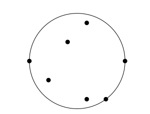
We can write this optimization problem as

$\minunder{(x,\, y)\in C}\; r, \tag{9.1}$

where

$C = \{(x, y)\in \RR^2 \mid (x - x_i)^2 + (y- y_i)^2 \leq r^2\quad\text{for}\quad i = 1, \dots, n\}.$ Upon rewriting this turns into the optimization problem

$\minunder{(x,\, y)\in C'}\; x^2 + y^2 + \lambda, \tag{9.2}$ where

$C' = \{(x, y, \lambda)\in \RR^3 \mid x_i^2 + y_i^2 \leq 2 x_i x + 2 y_i y + \lambda\quad \text{for}\quad i = 1, \dots, n\}$ and $\lambda = r^2 - x^2 - y^2$ .

Prove that (9.1) and (9.2) both are convex optimization problems. Explain how (9.1) is rewritten into (9.2) .

Hint

Expand

$(x - x_i)^2 + (y- y_i)^2 \leq r^2$ and put $\lambda = r^2-x^2-y^2$ .

The rewriting (9.2) may look unmotivated now, but it earns its keep in Section 9.3 , where an interior point method computes the optimal fire station location.

9.1 The optimal separating hyperplane

In section 5.3.2 we were presented with labeled data

$(v_1, y_1), \dots, (v_m, y_m), \tag{9.3}$ where $v_i\in \RR^d$ and $y_i = \pm 1$ . The task at hand was to separate differently labeled data by a hyperplane $\alpha^\top v + \beta = 0$ , such that

$\begin{aligned} \alpha^\top v_i + \beta &> 0\quad\text{if}\quad y_i = 1\\ \alpha^\top v_i + \beta &< 0\quad\text{if}\quad y_i = -1 \end{aligned}\tag{9.4}$ for $i = 1, \dots, m$ . Please browse back to Definition 4.40 for the definition of a hyperplane in $\RR^d$ .

Such a hyperplane need not exist: for the points $(1, 1), (-1, -1)$ with label $+1$ and $(-1, 1), (1, -1)$ with label $-1$ , the four inequalities in (9.4) contradict each other, as you showed in Exercise 5.9 . Separability is a genuine assumption on the data — we return to what can be done without it with the kernel functions of Section 9.2 .

If the data in (9.3) can be separated according to (9.4) , we may find a hyperplane $(\alpha^*)^\top x + \beta^* = 0$ , such that

$\begin{aligned} (\alpha^*)^\top v_i + \beta^* &\geq 1\quad\text{if}\quad y_i = 1\\ (\alpha^*)^\top v_i + \beta^* &\leq -1\quad\text{if}\quad y_i = -1. \end{aligned}\tag{9.5}$

How do you go from (9.4) to (9.5) ?

Suppose that

$\begin{aligned} \alpha^\top v_i + \beta &> 0\quad\text{if}\quad y_i = 1\\ \alpha^\top v_i + \beta &< 0\quad\text{if}\quad y_i = -1. \end{aligned}$ Let

$\begin{aligned} N &= \min\{\alpha^\top v_i + \beta \mid y_i = 1\}\\ M &= \max\{\alpha^\top v_i + \beta \mid y_i = -1\}. \end{aligned}$ Show that $N > 0$ and $M < 0$ . How can $N$ and $M$ be applied in constructing $\alpha^*$ and $\beta^*$ ?

Consider

$\begin{aligned} \alpha^\top v_i + \beta \geq N &> 0\quad\text{if}\quad y_i = 1\\ \alpha^\top v_i + \beta \leq M &< 0\quad\text{if}\quad y_i = -1. \end{aligned}$ What is special about $s = \min(N, |M|)$ ?

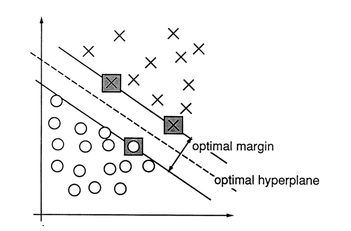
What does optimal hyperplane mean in this setting? It is the one maximizing the width of the strip between the two labeled clusters.

Figure from the Cortes and Vapnik paper: Support vector networks, Machine Learning, 1995.

The inequalities (9.5) describe this strip precisely. The two parallel hyperplanes

$H_{+}\colon\, \alpha^\top v + \beta = 1 \qquad\text{and}\qquad H_{-}\colon\, \alpha^\top v + \beta = -1$ bound a strip containing no data points: by (9.5) the points labeled $+1$ lie on or beyond $H_{+}$ and the points labeled $-1$ on or beyond $H_{-}$ . The separating hyperplane $H$ given by $\alpha^\top v + \beta = 0$ runs down the middle of the strip. This is exactly the picture above: $H$ is the solid line, $H_{+}$ and $H_{-}$ the dashed ones.

Here lies a crucial insight, only implicit in the paper by Cortes and Vapnik: the normalization to $\pm 1$ in (9.5) costs nothing — rescale $\alpha$ and $\beta$ , as in the exercise above — and it makes the width of the strip visible in $\alpha$ alone.

Indeed, the distance from a point $u$ to the hyperplane $H$ is

$\frac{|\alpha^\top u + \beta|}{|\alpha|}$ by Exercise 9.7 below. A point $u$ on $H_{+}$ satisfies $\alpha^\top u + \beta = 1$ and therefore has distance $1/|\alpha|$ to $H$ , and the same holds on $H_{-}$ . The strip therefore has width

$\frac{1}{|\alpha|} + \frac{1}{|\alpha|} = \frac{2}{|\alpha|},$ and the optimal hyperplane is the one making $|\alpha|$ as small as possible subject to (9.5) . Since minimizing $|\alpha|$ is the same as minimizing $|\alpha|^2$ — and the square is a differentiable (convex!) function — we have arrived at a convex optimization problem.

Let $H$ be the hyperplane in $\RR^d$ given by $\alpha^\top v + \beta = 0$ and let $u\in \RR^d$ . The point closest to $u$ in $H$ can be found by solving the optimization problem

$\minunder{v\in H}\; |v - u|^2. \tag{9.6}$

Explain why (9.6) is a convex optimization problem.

Show how Theorem 7.39 can be used to solve this optimization problem by first deducing the equations

$\begin{aligned} -2(u - v) + \lambda \alpha &= 0\\ \alpha^\top v + \beta &= 0 \end{aligned}\tag{9.7}$ for the Lagrange multiplier $\lambda$ . Notice here that $-2(u-v) + \lambda \alpha = 0$ above really contains $d$ equations, whereas $\alpha^\top v + \beta = 0$ is only one equation in $x_1, \dots, x_d$ , where $v = (x_1, \dots, x_d)^\top$ . Solve the equations (9.7) for $v\in \RR^d$ and $\lambda\in \RR$ . How can we be sure that $v$ really is a minimum in (9.6) ?

Finally show that the distance from $H$ to $u$ is given by the formula

$\left| \frac{\alpha^\top u + \beta}{|\alpha|}\right|.$

Summing up, we have proved the following result.

Let the points $v_1, \dots, v_m\in \RR^d$ be labeled by $y_1, \dots, y_m\in \{\pm 1\}$ . Then the optimal hyperplane $H=\{v\in \RR^d\mid \alpha^\top v + \beta = 0\}$ separating the points is given by the optimization problem

$\minunder{\alpha^\top v_i + \beta\, \geq\, 1 \;\text{if}\; y_i = 1\\[2pt] \alpha^\top v_i + \beta\, \leq\, -1 \;\text{if}\; y_i = -1}\; |\alpha|^2$ for $i = 1, \dots, m$ .

The vectors $v_i$ among the data points $v_1, \dots, v_m$ satisfying $\alpha^\top v_i + \beta = 1$ or $\alpha^\top v_i + \beta = -1$ are called support vectors.

An optimal solution always has support vectors. If no data point satisfied its constraint with equality, all the numbers $|\alpha^\top v_i + \beta|$ would exceed $1$ by a common factor $s > 1$ , and dividing both $\alpha$ and $\beta$ by $s$ would preserve the constraints in Theorem 9.8 while shrinking $|\alpha|$ — so the strip was not the widest after all. A little more thought (shift $\beta$ to re-center the strip, then rescale) shows that both dashed lines must carry support vectors, just as in the figure above.

Let us explicitly write up the optimization problem in Theorem 9.8 in a very simple situation: finding the best line $y = a x + b$ separating the points $(1, 1)$ and $(2, 2)$ . In the notation of (9.5) , we have (without the stars on $\alpha$ and $\beta$ )

$\alpha = \begin{pmatrix} a \\ -1 \end{pmatrix}\qquad\text{and}\qquad \beta = b$ so that

$\alpha^\top \begin{pmatrix} x \\ y \end{pmatrix} + b = a x - y + b = 0.$ The points are

$v_1 = \begin{pmatrix} 1 \\ 1 \end{pmatrix}\qquad\text{and}\qquad v_2 = \begin{pmatrix} 2 \\ 2 \end{pmatrix},$ where $y_1 = 1$ and $y_2 = -1$ .

Therefore the optimization problem in Theorem 9.8 becomes

$\minunder{a + b\, \geq\, 2\\[2pt] 2 a + b\, \leq\, 1}\; 1 + a^2. \tag{9.8}$

Solve the optimization problem (9.8) and verify that the best line from the optimization problem is the one we expect it to be. Also, check how WolframAlpha solves this optimization problem.

Hint

You could maybe use Fourier-Motzkin elimination to show that

$\begin{aligned} a + b &\geq 2\\ 2 a + b&\leq 1 \end{aligned}$ implies $a \leq -1$ .

Notice that the optimization problem in Theorem 9.8 has number of constraints equal to the number of points to be separated. Notice also that it has no solution at all when the data cannot be separated — the constraints are then contradictory. The remedy, called the soft margin, is stated precisely when we meet the parameter C of sklearn in the next section.

Usually one does not use the optimization problem in Theorem 9.8 , but rather its socalled (Lagrange) dual for finding the optimal hyperplane. This dual optimization problem uses that the normal vector $\alpha$ is a linear combination

$\alpha = \lambda_1 y_1 v_1 + \cdots + \lambda_m y_m v_m \tag{9.9}$ of the support vectors weighted by their labels. It is an optimization problem in $\Lambda^\top = (\lambda_1,\dots, \lambda_m)$ from (9.9) and looks like

$\maxunder{\Lambda\, \geq\, 0\\[2pt] \Lambda^\top Y\, =\, 0}\; \lambda_1 + \cdots + \lambda_m - \frac{1}{2} \Lambda^\top D \Lambda, \tag{9.10}$ where $Y =(y_1, \dots, y_m)^\top$ is the vector of labels attached to the points $v_1, \dots, v_m$ and $D$ is the symmetric $m\times m$ matrix given by

$D_{ij} = y_i y_j\, v^\top_i v_j = y_i y_j\, v_i\cdot v_j. \tag{9.11}$

Notice that the dual optimization problem is an optimization problem in $\RR^m$ , where $m$ is the number of data points. This can be in stark contrast to the original optimization problem in Theorem 9.8 , which is an optimization problem in $\RR^d$ , where $d$ is the dimension of the data points. Sometimes the data points are high dimensional and it pays to solve the dual optimization problem.

Let us write down the dual optimization problem for the points in Example 9.9 . Here

$\Lambda = \begin{pmatrix} \lambda_1 \\ \lambda_2 \end{pmatrix}, \quad Y = \begin{pmatrix} 1 \\ -1 \end{pmatrix}\quad \text{and}\quad D = \begin{pmatrix} 2 & -4 \\ -4 & 8 \end{pmatrix}$ so that the dual optimization problem becomes

$\maxunder{\lambda_1\, \geq\, 0,\;\; \lambda_2\, \geq\, 0\\[2pt] \lambda_1 - \lambda_2\, =\, 0}\; \lambda_1 + \lambda_2 -\lambda_1^2 - 4 \lambda_2^2 + 4\lambda_1 \lambda_2.$ This reduces to the optimization problem of maximizing $2 \lambda - \lambda^2$ subject to $\lambda \geq 0$ , which has the solution $\lambda = 1$ . Therefore the optimal hyperplane has normal vector

$\alpha = \lambda_1 y_1 \begin{pmatrix} 1 \\ 1 \end{pmatrix} + \lambda_2 y_2 \begin{pmatrix} 2 \\ 2 \end{pmatrix} = \begin{pmatrix} 1 \\ 1 \end{pmatrix} - \begin{pmatrix} 2 \\ 2 \end{pmatrix} = \begin{pmatrix} -1 \\ -1 \end{pmatrix}.$ The constraints hold with equality at the two support vectors, so $\beta = 3$ and the optimal hyperplane is the line $x + y = 3$ — the perpendicular bisector between the two points, exactly as geometry demands.

The dual optimization problem (9.10) can be derived formally from the original optimization problem in Theorem 9.8 . This is, however, beyond the scope of this course (see section 2.1 of the Cortes and Vapnik paper).

9.2 Support vector machines

The optimization problem of Theorem 9.8 , its dual (9.10) and the kernel functions introduced below make up one of the most celebrated algorithms of machine learning: the support vector machine (SVM) from the Cortes and Vapnik paper cited above. You do not have to implement it yourself: the python library sklearn ships an industrial implementation in sklearn.svm, and with kernel="linear" and a very large parameter C it solves exactly the optimization problem of Theorem 9.8 . The parameter C is the price of violating the margin, and we can say precisely what that means: for any labeled data — separable or not — sklearn solves the soft margin problem

$\minunder{y_i (\alpha^\top v_i + \beta)\, \geq\, 1 - \xi_i\\[2pt] \xi_i\, \geq\, 0}\; \frac{1}{2}|\alpha|^2 + C\, (\xi_1 + \cdots + \xi_m)$ for $i = 1, \dots, m$ , from section 3 of the Cortes and Vapnik paper. The new slack variable $\xi_i$ measures how far the point $v_i$ falls short of its margin constraint (for $\xi_i = 0$ the constraint is Theorem 9.8 's, with the two label cases abbreviated into one inequality), and the objective charges $C$ per unit of shortfall. A huge C makes slack unaffordable and recovers the hard margin of Theorem 9.8 ; a moderate C buys a wider strip on messy data, at the price of points inside the strip or even on the wrong side — the Gaussian kernel cell later in this section runs with C=10 in exactly this spirit. In the dual, C shows up as the extra constraint $\lambda_i \leq C$ : a cap on how much influence any single data point can buy.

Three small observations that explain what sklearn is doing.

Check that for $\xi_i = 0$ the constraint $y_i(\alpha^\top v_i + \beta) \geq 1 - \xi_i$ is exactly the constraint of Theorem 9.8 , for both values of the label $y_i$ .
Show that the soft margin problem is feasible for any labeled data — no separability needed. So unlike the problem in Theorem 9.8 , it always has something to optimize.
Suppose the data can be separated, and let $(\alpha^*, \beta^*)$ be the optimum of Theorem 9.8 . Show that the slack at the soft margin optimum satisfies
$\xi_1 + \cdots + \xi_m \leq \frac{|\alpha^*|^2}{2C},$ so the total slack vanishes as $C$ grows — the hard margin reappears.

Hint

For the second part: $\alpha = 0$ , $\beta = 0$ and $\xi_i = 1$ satisfy every constraint. For the third: $(\alpha^*, \beta^*)$ with all $\xi_i = 0$ is one candidate in the soft margin problem, so the optimum costs at most $\frac{1}{2}|\alpha^*|^2$ — and the term $C(\xi_1 + \cdots + \xi_m)$ is part of that cost.

9.2.1 Two clusters in the plane

The cell below separates two clusters of points. It prints the optimal $\alpha$ and $\beta$ , draws the optimal hyperplane (solid) with the two margin lines $\alpha^\top v + \beta = \pm 1$ (dashed), and circles the support vectors. Look closely at the printed numbers: at the support vectors, $\alpha^\top v_i + \beta$ equals $\pm 1$ exactly — these are the constraints of Theorem 9.8 holding with equality, computed numerically.

Live Python

import numpy as np
import matplotlib.pyplot as plt
from sklearn import svm

blue = np.array([[1.0, 2.0], [1.5, 2.8], [2.0, 2.2], [1.2, 3.2], [0.8, 2.6]])
red  = np.array([[3.2, 0.6], [3.8, 1.4], [4.4, 0.8], [3.5, 0.2], [4.1, 1.8]])

X = np.vstack([blue, red])
y = np.array([1]*len(blue) + [-1]*len(red))

model = svm.SVC(kernel="linear", C=1e6)   # huge C: hard margin
model.fit(X, y)

alpha, beta = model.coef_[0], model.intercept_[0]
print("alpha =", np.round(alpha, 4), "  beta =", round(beta, 4))
sv = model.support_vectors_
print("alpha^T v + beta at the support vectors:", np.round(sv @ alpha + beta, 4))

g1, g2 = np.meshgrid(np.linspace(0, 5, 300), np.linspace(-0.5, 4, 300))
z = (np.column_stack([g1.ravel(), g2.ravel()]) @ alpha + beta).reshape(g1.shape)

plt.contour(g1, g2, z, levels=[-1, 0, 1],
            colors="gray", linestyles=["dashed", "solid", "dashed"])
plt.scatter(*blue.T, color="blue", s=40)
plt.scatter(*red.T, color="red", s=40)
plt.scatter(*sv.T, s=180, facecolors="none", edgecolors="black")
plt.gca().set_aspect("equal")
plt.show()

Only the circled points matter: move any other point a little (rerun and try!) and the optimal hyperplane does not budge. The hyperplane is carried entirely by its support vectors — hence the name.

Suppose the labeled points $v_1, \dots, v_m\in \RR^d$ can be separated by a hyperplane. Which of the following statements are true?

The optimal separating hyperplane is completely determined by its support vectors.

Any four points in the plane, two labeled $+1$ and two labeled $-1$ , can be separated by a line.

The dual optimization problem (9.10) has one variable per data point.

Moving any of the data points a little always changes the optimal hyperplane.

9.2.2 Reading handwritten digits

Support vector machines are not a museum piece. Before the deep learning era they were the state of the art for tasks like text classification and protein classification, and for small data sets with many measurements per data point they remain a favorite — this is exactly the situation of Remark 9.11 , where the dual problem has one variable per data point rather than one per dimension.

Here is an example you already know: the $8\times 8$ handwritten digits that the neural network of Section 7.9 read in the previous chapter — every digit its vector of $64$ pixel values, a data point in $\RR^{64}$ . We ask the machine the honest yes/no question of practice: is this digit a $5$ ? Label every $5$ with $+1$ and everything else with $-1$ , and Theorem 9.8 applies unchanged. Note what just happened: the "two clusters" of the theorem are two labels, nothing more. The $-1$ class is a motley union of nine kinds of digit, and the mathematics does not blink — the two-blob pictures we have drawn are visual aids, not hypotheses. This one-against-the-rest trick is also how binary classifiers handle many classes in practice: train ten machines, one per digit, and let the largest decision value win.

It is far from obvious that a single hyperplane in $\RR^{64}$ can separate the fives from the nine-digit crowd — but for these $1500$ training digits it can, so we demand the hard margin (a huge C) and get exactly the optimal hyperplane of Theorem 9.8 .

The best part is the picture: the support vectors are themselves digits, and they are the machine's entire concept of five-ness. The optimization problem singles out a handful of borderline fives (top row below) together with a gallery of five-impersonators — digits of other classes that flirt with looking like a $5$ , shown with their true labels in the middle row. When we ran it, the impersonators were mostly 9s, 7s, 3s and 6s: exactly the digits that share strokes with a five. The bottom row shows some of the ignored, neatly written majority — move any of those and the hyperplane does not budge. The cell prints your exact counts, which may drift slightly with the library version.

Better still, the number $\alpha^\top v + \beta$ measures how manifestly a digit is a $5$ . Recall from (9.5) that the optimal hyperplane was normalized to give values $\geq 1$ on one cluster and $\leq -1$ on the other, with the margin strip $-1 < \alpha^\top v + \beta < 1$ in between. So a digit with $\alpha^\top v + \beta \geq 1$ is manifestly a five — it clears the margin — while a value near $0$ means the machine is honestly unsure. The cell sorts the $297$ unseen digits by $\alpha^\top v + \beta$ and displays the extremes and the ambiguous middle. When we ran it, every unseen five landed on the correct side — nearly all manifestly, a couple hesitantly inside the margin — at the price of a couple of false alarms among the non-fives; again the cell prints your exact counts.

Live Python

import numpy as np
import matplotlib.pyplot as plt
from sklearn import svm
from sklearn.datasets import load_digits

digits = load_digits()               # the 8x8 digits from Chapter 7
X = digits.data
y = np.where(digits.target == 5, 1, -1)   # a 5, or not a 5

Xtr, Xte = X[:1500], X[1500:]             # train on 1500 digits ...
ytr, yte = y[:1500], y[1500:]             # ... test on the 297 others
ttr = digits.target[:1500]                # true digits, for the titles

model = svm.SVC(kernel="linear", C=1e6)   # huge C: hard margin
model.fit(Xtr, ytr)

sv = model.support_
fives = [i for i in sv if ttr[i] == 5]
imps  = [i for i in sv if ttr[i] != 5]
rest  = [i for i in range(len(Xtr)) if i not in sv]
print(f"support vectors: {len(sv)} of 1500 training digits "
      f"({len(fives)} borderline 5s + {len(imps)} impersonators)")

f = model.decision_function(Xte)          # alpha^T v + beta
print("errors on the unseen digits:", (np.sign(f) != yte).sum())
print("unseen 5s clearing the margin (f >= 1):",
      ((f >= 1) & (yte == 1)).sum(), "of", (yte == 1).sum())

# rows: borderline 5s | 5-impersonators | ignored crisp majority
fig, axes = plt.subplots(3, 8, figsize=(8, 4))
for ax in axes.ravel():
    ax.axis("off")
for ax, i in zip(axes[0], fives):
    ax.imshow(Xtr[i].reshape(8, 8), cmap="gray_r")
    ax.set_title("5", fontsize=8)
for ax, i in zip(axes[1], imps):
    ax.imshow(Xtr[i].reshape(8, 8), cmap="gray_r")
    ax.set_title(int(ttr[i]), fontsize=8)
for ax, i in zip(axes[2], rest):
    ax.imshow(Xtr[i].reshape(8, 8), cmap="gray_r")
    ax.set_title(int(ttr[i]), fontsize=8, color="gray")
plt.show()

# the unseen digits sorted by f: manifestly not 5 ... manifestly 5
order = np.argsort(f)
picks = np.r_[order[:5], np.abs(f).argsort()[:6], order[-5:]]
fig, axes = plt.subplots(1, 16, figsize=(10.5, 1.5))
for ax, i in zip(axes, picks):
    ax.imshow(Xte[i].reshape(8, 8), cmap="gray_r")
    ax.set_title(f"{f[i]:.1f}", fontsize=7)
    ax.axis("off")
plt.show()

Study the strip: on the far left (large negative $\alpha^\top v + \beta$ ) unmistakably not fives, on the far right textbook fives, and in the middle handwriting that would make a human hesitate too. Note the family resemblance to the Challenger neuron of the previous chapter: there the same affine expression was fed through the sigmoid to become a probability; here it is left raw and read against the margin.

Compare with the previous chapter, too: there, reading digits took a $2410$ -parameter neural network and thousands of gradient descent steps. Here the single yes/no question is it a five? is answered by one convex optimization problem carried by a few dozen support vectors, with the guarantee from Theorem 6.13 that the hyperplane found is globally optimal.

9.2.3 Separating sentences

Digits were easy to feed to the machine: an image is born a vector. But most of what the world wants classified is text — support requests, product reviews, spam. Chapter 5 already showed the way in: after the one-hot encoding (5.16) came its modern replacement, the folded cell of $18$ words embedded by the small language model all-MiniLM-L6-v2 — the model behind Ask the book on this very page — which turns any sentence into a learned vector in $\RR^{384}$ whose geometry carries meaning.

That is one half of the modern recipe for classifying text. The other half is this chapter. Take a big pretrained model, freeze it, embed your sentences, and train nothing but a separating hyperplane on the resulting vectors. Practitioners call this a linear probe, and it is everyday industrial machine learning: under many a spam filter, content moderator and ticket router sits exactly the soft-margin problem of Exercise 9.13 , working on top of somebody else's embeddings.

Let us run the recipe, honestly and end to end. The task: do film reviews express enthusiasm or disappointment? Below are $46$ short reviews written for this book — the first $20$ enthusiastic, the next $20$ disappointed, and a final $6$ held back as unseen test sentences. A language model is far too large to run inside a web page, so the reviews were embedded once, in advance, and their vectors travel with this page exactly like the $18$ words of Chapter 5: $8$ -bit integers, one scaling factor per vector. Open the fold and you are looking at rows of $\RR^{384}$ ; run the cell to decode them into the matrix VECS.

Python: 46 film reviews as learned vectors in dimension 384

Live Python

import numpy as np

# 46 short film reviews embedded by all-MiniLM-L6-v2 (unit length,
# stored as integers): rows 0-19 enthusiastic, 20-39 disappointed,
# 40-45 held back for testing.
REVIEWS = [
    "An absolute joy from the first minute to the last.",
    "I laughed, I cried, and I bought a ticket for the next night.",
    "A masterpiece — the best film I have seen in years.",
    "Gorgeous photography and a story that stays with you.",
    "The whole cinema burst into applause at the end.",
    "Smart, funny and full of heart.",
    "Two hours flew by; I did not look at my phone once.",
    "The soundtrack alone is worth the price of admission.",
    "A warm, generous film that trusts its audience.",
    "Easily the most fun I have had at the movies this year.",
    "Not bad at all — in fact I liked it far more than I expected.",
    "It starts slowly, but the ending makes up for everything.",
    "Every scene is composed like a painting.",
    "I hugged a stranger on the way out; it is that kind of film.",
    "Finally a sequel that surpasses the original.",
    "The children were spellbound and so was I.",
    "Funny without being silly, moving without being sentimental.",
    "I will be thinking about that last shot for weeks.",
    "Three hours long and I wished it were longer.",
    "The rare comedy that actually made me laugh out loud.",
    "A complete waste of two hours of my life.",
    "The plot makes no sense and the dialogue is even worse.",
    "I walked out halfway through, and I never walk out.",
    "Dull, predictable and about forty minutes too long.",
    "The trailer contained every good scene in the film.",
    "I have seen commercials with more emotional depth.",
    "The lead actor looked as bored as I felt.",
    "Save your money and stay home.",
    "A tired copy of a dozen better films.",
    "By the end I was cheering for the villain out of spite.",
    "It was fine, I suppose, but I had forgotten it by dinner.",
    "Beautiful to look at, yet somehow completely empty.",
    "The jokes landed with the grace of a falling piano.",
    "I checked my watch eleven times; I counted.",
    "How do you make a dinosaur film boring? Watch and learn.",
    "The romance had all the chemistry of a tax form.",
    "Half the audience was asleep by the second act.",
    "A two-hour trailer for a film that never arrives.",
    "My popcorn was more memorable than the plot.",
    "Even the outtakes during the credits fell flat.",
    "I want to watch it again tomorrow.",
    "My whole family loved every minute of it.",
    "A small film with a huge heart — go see it.",
    "Honestly, I nearly fell asleep before the intermission.",
    "The book was wonderful; this film is an insult to it.",
    "Ninety minutes I will never get back.",
]

SCALES = [0.00134925, 0.00134631, 0.00166664, 0.00120350,
          0.00113177, 0.00145875, 0.00131503, 0.00132865,
          0.00129732, 0.00158051, 0.00139407, 0.00150941,
          0.00138658, 0.00109629, 0.00119279, 0.00108930,
          0.00116800, 0.00136563, 0.00181498, 0.00110403,
          0.00122117, 0.00139232, 0.00133934, 0.00137679,
          0.00143937, 0.00131870, 0.00115037, 0.00139765,
          0.00113222, 0.00142804, 0.00143683, 0.00142923,
          0.00129417, 0.00106869, 0.00152763, 0.00144977,
          0.00139511, 0.00136846, 0.00103306, 0.00134011,
          0.00167615, 0.00127986, 0.00115027, 0.00116656,
          0.00132876, 0.00183315]

RAW = """
2 8 -26 -94 17 50 5 -6 58 2 20 -7 42 -10 -23 -9 -6 -53 4 23 17 39 3 46 -18 34 5 1 40 -50 -32 -46 93 41 -34 -15 -5 -40 28 -8 38 -68 4 32 -3 53 35 -33 96 36 23 -14 -5 -36 7 21 28 -28 -58 21 2 37 -2 14 30 -108 11 -11 4 46 1 -3 24 -27 -48 -10 3 -19 17 18 28 -66 23 11 -17 -52 10 -4 28 3 -116 0 -64 -26 -27 -4 6 -45 12 55 -40 3 -6 -3 20 -33 -24 42 7 -45 -33 -25 52 -3 43 6 -35 31 18 8 59 36 -38 -16 4 -7 19 0 6 23 34 41 -12 12 -2 -13 -71 72 -37 50 -8 -44 -21 -63 -96 -20 -22 17 -26 28 39 -4 -8 9 -5 -27 -8 -2 -48 7 -101 -28 -17 -7 -38 -21 17 23 -35 -8 -4 12 -8 32 -3 105 -36 19 -2 -33 94 27 -4 29 6 -36 -14 -10 28 11 0 -20 -21 13 19 -7 52 -23 22 -23 -14 -89 -4 9 3 -68 22 -16 18 -23 -7 -46 78 0 24 -41 -79 9 -21 -13 127 18 -33 0 52 -37 -13 83 -2 -1 22 108 -97 62 25 -3 34 8 -48 17 104 3 41 -7 40 44 -26 -10 -40 30 50 -26 -75 -74 59 -7 -47 -34 -31 41 51 42 -16 49 10 4 -6 43 48 4 11 3 -57 19 -12 -16 -13 -38 -13 -25 -26 6 99 -45 -46 11 7 -12 9 10 0 38 -15 4 -56 70 -24 19 -10 3 1 -5 -23 -72 -62 -10 5 -2 -48 42 -4 -11 64 29 -14 58 -22 49 42 0 1 56 -88 -35 -7 26 6 -24 -20 -31 78 65 30 -1 -3 18 56 -25 28 22 14 32 -15 -44 -20 16 -14 -34 -6 -20 32 8 -47 14 -92 33 32 39 -16 -50 -26 43 -52 3 -64 -30 61 23 41 3 15 -36 6 70 70 -33 -6 -2 -58 78 19 24 -7 43
23 6 20 -33 23 -28 43 34 -8 -43 -21 12 18 51 -13 -20 -28 -34 -4 3 -17 12 -46 54 -12 4 3 -51 -30 -11 -22 -13 -9 17 22 -59 14 -70 48 36 38 -29 19 45 75 2 24 17 106 -19 26 1 6 -83 -20 17 23 4 -11 2 8 -4 15 34 -74 -30 -23 -22 41 61 67 1 30 26 -31 70 15 -17 21 52 -49 -80 -23 -54 67 -69 24 48 -33 11 53 -52 -13 44 -25 -10 -20 31 19 36 10 31 43 -40 34 -22 -42 34 12 -71 -15 47 18 16 -58 66 -40 6 25 -45 36 35 7 47 15 -46 8 0 -18 -18 6 -29 84 28 -17 -23 -88 49 -58 -28 -25 -41 13 33 -53 23 18 9 -9 27 -5 24 -31 31 -9 -59 127 14 -50 13 54 54 -5 28 -19 9 -52 -35 -23 -11 -23 27 -30 25 -85 5 86 -16 -50 29 28 -25 31 -17 44 -17 5 -19 -22 -19 17 29 -69 -21 -31 -60 16 -78 58 -1 32 -20 -21 13 -33 -22 21 -45 50 -44 -4 20 77 13 38 -83 -39 -46 -5 -32 79 -43 63 0 38 9 -41 -29 -19 -26 0 49 36 22 30 4 40 39 26 -98 40 -2 -7 14 -5 11 29 4 -35 3 72 16 -34 -39 13 -57 -52 3 43 43 43 -5 -49 -39 -8 -5 41 77 14 -2 9 -18 17 15 -47 15 1 7 -33 -9 -4 22 53 -44 -86 -12 -67 26 -15 -55 14 -1 -18 41 -8 23 -6 80 50 -30 -15 93 -23 -19 13 2 4 13 -42 19 47 -24 -54 84 -12 30 9 -17 1 0 -24 52 -90 -25 25 -34 3 18 -108 18 24 63 -4 -4 -39 11 77 -22 21 -19 -33 40 -15 10 -5 27 -32 17 28 -5 -14 31 -29 9 -47 -67 8 -36 100 25 -57 -19 -3 -20 33 39 0 20 51 10 -7 -27 -78 41 48 -45 -22 6 -6 33 -22 -43 -56 28
-43 33 4 -31 -32 44 -22 27 -5 -25 -37 33 25 40 -17 56 40 -61 60 -54 10 11 9 32 -36 29 18 28 -54 0 11 24 -26 -3 6 19 -1 -20 -23 -40 -8 -25 19 -35 17 -36 -2 -16 48 -13 -24 37 2 -23 0 -28 -22 -29 9 -48 -27 -1 4 11 20 -41 -3 -19 -30 50 -15 18 28 -21 -27 -49 -21 -33 -18 -27 25 -32 -20 16 20 -19 54 23 -25 47 -28 -20 -50 25 5 -41 -19 -31 -1 38 -2 -5 -44 -51 50 -41 70 17 -9 -24 7 -24 9 33 23 -11 1 -5 -8 51 52 29 -13 35 -41 -63 48 0 -29 13 25 55 13 -8 -13 37 -61 14 -14 -30 -23 2 24 33 -16 -8 23 -6 -42 44 -17 -27 -27 -10 -7 9 3 5 24 13 -39 -15 15 1 -14 -11 39 36 -43 4 -49 36 17 46 35 30 15 24 2 -19 -28 3 -33 36 15 27 65 -20 12 45 -57 28 5 68 13 22 -13 8 -65 -23 10 -72 58 -4 23 -5 -19 -9 -27 40 5 -12 -1 21 -29 -57 1 36 -1 -50 41 -7 -35 0 38 -25 8 27 -28 -18 -127 35 -9 -5 -6 -6 30 25 0 24 30 -47 -10 10 -1 29 25 -35 -31 35 -17 2 15 -23 -6 -16 -29 -22 -31 59 27 -47 -13 54 -8 12 -5 51 14 -8 -1 24 -15 9 -45 43 -26 -32 -2 -15 -12 -30 26 6 -21 -24 -75 10 -9 25 8 15 -35 21 -44 -5 -45 39 8 2 46 -23 9 -4 -22 -21 7 12 27 70 -5 -37 0 45 14 12 28 -37 15 0 -7 26 -44 -33 -22 -44 -2 6 -10 -8 -26 4 -7 6 -32 19 67 -18 15 36 -1 -23 41 -22 -30 22 -13 -63 5 25 26 27 -1 31 -13 -11 14 0 9 -83 25 60 -37 -23 36 42 72 -31 -37 17 9 -9 36 61 48 2 -24 -13 -46 8 82 2 20 -1
-25 58 54 34 19 -9 50 -47 12 -10 37 93 63 12 -35 28 23 -50 -20 4 -104 42 39 11 -25 14 23 -7 -10 -46 -44 37 -42 26 -8 29 13 -76 12 -11 -9 -5 37 24 -27 -16 6 -27 -11 19 -50 -18 -20 -23 -28 36 -52 -58 18 -56 28 86 -23 69 55 16 -43 25 46 -42 -51 72 -38 35 -32 -26 2 -83 8 -12 62 -28 -7 20 -37 -127 41 -51 -10 -25 -24 -49 -28 -39 -73 -27 -40 -44 -25 28 15 -1 3 42 35 7 -28 1 -11 -2 21 52 -67 41 70 -4 -24 45 67 -3 47 7 -50 27 -59 -63 98 0 9 37 44 108 86 -6 -33 52 -121 13 16 51 -8 39 12 -12 -37 2 62 73 -38 -44 -8 75 -43 16 47 -16 9 8 -38 81 33 -60 22 -49 -44 -90 68 73 -25 37 -66 -16 48 45 -14 94 -34 -9 -52 -26 -32 4 -49 -25 -7 -46 16 -15 115 24 -78 -43 46 2 27 20 -36 50 -73 21 42 -20 -18 -7 -29 -35 10 57 6 51 -54 -21 2 -29 -4 -67 -58 13 41 32 61 -50 22 0 45 38 32 6 50 -48 -64 63 15 64 -7 -2 -28 -46 -68 -54 60 -85 -106 26 15 32 -17 -15 -35 55 -3 0 9 -23 6 3 34 -46 -16 53 38 -24 -21 58 10 -46 23 14 24 -40 23 24 -13 -15 -26 12 20 12 -16 -37 -3 9 71 29 -93 45 -67 27 13 -30 24 -34 -69 35 -14 -26 38 47 6 -66 7 -37 6 -9 -34 -52 -3 17 57 8 -25 -71 -3 -37 -10 28 -24 -54 45 0 -13 -14 -49 -61 30 -37 92 1 -23 31 -10 -25 0 27 -40 -41 72 59 6 54 39 -34 27 -5 -83 3 10 -4 17 -5 25 47 53 39 -18 -22 6 -41 -6 -52 -26 47 -8 43 19 -8 107 -33 -46 68 -40 -48 32 90 -14 -52 17 9 -9 47 78 -13 -119 36
4 15 12 -31 48 59 14 20 69 -71 38 11 -7 1 -39 -1 48 -21 20 -11 29 67 33 76 -16 -4 19 -36 -15 4 28 10 22 14 -23 -11 7 10 -13 -26 -22 -64 48 8 63 -37 6 -52 119 22 -28 3 -3 -56 52 -61 55 -47 26 -64 -15 14 -26 2 69 -51 25 10 -27 109 10 -18 65 -27 -34 12 -35 -37 -16 9 37 -111 -60 -35 35 -22 71 26 -65 78 -122 -46 -79 42 34 -69 -20 -88 114 9 -21 -13 4 -36 12 -50 -23 39 -17 -13 -67 -31 63 0 82 42 -30 -21 -55 25 82 25 -97 30 12 -44 -10 0 -30 -17 29 -5 23 38 6 46 -24 21 -34 -7 -6 -42 -36 -3 -10 57 -50 -6 -46 110 -37 52 -30 -13 17 71 -2 19 7 6 23 2 41 -62 -26 -22 -6 -9 -22 35 -71 22 -93 64 -37 8 39 93 -4 0 50 9 -39 55 26 1 9 -69 -35 22 -5 -27 -95 63 -13 -2 -15 14 -64 -1 -37 5 -47 26 -44 6 80 -19 -5 6 54 -28 74 18 -35 -65 -41 32 -35 -48 80 16 -40 0 105 11 -125 -8 -12 21 -82 48 -18 13 61 -6 27 9 -47 -38 84 -6 31 115 25 -34 74 -67 7 47 -48 13 16 -39 54 -46 -88 -6 -67 66 42 -21 16 1 -7 -46 -47 69 38 -26 18 49 -56 -15 -97 -26 67 -52 -30 12 30 34 18 -71 -36 16 -7 -50 13 23 34 32 1 -17 9 26 -62 56 -46 35 -16 -4 38 -48 -44 -19 27 14 -41 28 37 -47 16 55 -9 31 117 -28 12 0 -79 26 -65 -67 35 -60 1 125 32 27 -9 31 47 33 -94 57 50 -63 9 -15 2 -14 42 -30 -9 37 -36 -6 -57 -38 15 -60 -127 -27 -60 105 70 -4 120 -27 17 0 13 25 43 70 69 -28 -4 -29 6 -16 -69 -35 52 -48 -19 74 -1 15 17 3 -16 41
-19 -34 27 -4 -35 -32 38 -5 24 46 -4 -36 -51 -19 3 -5 50 -96 0 -10 -34 19 12 -39 -54 8 10 -15 -28 40 14 -18 7 11 -9 15 11 58 21 -23 -17 -57 14 59 13 -62 21 -41 -25 42 -42 14 -42 47 16 11 -53 15 -22 22 -6 5 -7 21 24 -8 -59 15 -23 -17 43 10 -59 15 7 -31 3 -65 5 39 -14 -44 -71 -21 42 -55 -13 -45 -22 29 31 30 62 14 23 2 66 -40 -67 61 41 19 18 48 56 21 -18 26 -10 -68 40 -19 18 6 103 24 -17 37 15 -25 40 43 -8 0 -16 -23 18 0 -36 57 32 21 -25 53 23 20 -14 -12 4 27 -97 76 -84 53 -46 33 -34 48 15 6 -40 36 -12 -32 67 -2 -21 1 -26 40 -2 0 -10 -46 -58 -64 4 23 19 -14 -17 43 -21 -33 3 52 2 -1 -19 10 -36 10 -23 5 57 38 -38 -33 38 50 -9 -25 -15 4 -20 0 50 18 23 20 34 45 -127 22 32 -72 -14 -17 17 46 -26 -36 -12 -11 10 -61 -5 5 -21 11 52 -54 15 0 -13 -14 -8 9 20 -14 -29 34 56 66 -7 -1 -18 -33 17 -12 15 -90 -30 59 39 26 -27 70 -42 20 -2 -15 -36 -22 -3 33 -41 -15 -35 53 -32 -35 22 17 -32 -31 10 31 16 6 43 8 -42 -32 -52 48 -25 -2 24 -11 26 34 58 -29 -46 -2 58 23 -44 -19 -35 36 -77 -59 39 8 13 7 -50 7 -33 -22 40 -28 -36 -16 -14 -2 -34 37 -30 -9 29 -42 21 14 -36 -4 -44 0 9 -28 -48 -43 -45 22 -32 11 -24 -5 51 53 0 13 38 -14 -10 35 14 21 49 -12 -17 32 -19 -7 56 -26 16 108 -10 22 -46 -19 28 13 -38 -34 5 75 15 76 -25 -41 -21 -2 11 -10 2 44 13 -6 13 16 7 -25 -5 47 -45 29 73 4 50 -6
15 18 78 -15 69 -82 0 -3 33 -24 39 36 43 -28 -53 -31 -6 -81 -70 -15 23 30 -6 40 55 42 -19 17 -18 -27 -42 89 -42 77 29 -60 31 13 13 -51 6 22 78 20 18 -25 16 -18 29 2 -62 15 0 -14 -49 65 -19 32 24 10 -1 38 -1 18 -54 55 -47 -96 63 27 5 51 -15 42 -23 4 88 -79 36 -21 -12 -50 5 37 67 -25 -1 48 -44 -7 -6 -31 -46 -52 -48 -45 -46 11 -48 28 -20 29 17 27 25 2 9 -37 26 20 25 -29 46 42 -25 13 -11 55 43 5 23 -6 22 -65 -48 -66 38 0 -10 -4 6 45 -4 -17 -41 24 19 44 -19 13 34 -13 13 18 47 -12 -1 -35 -21 -112 -30 -35 37 7 45 -50 65 30 -52 15 -16 41 27 7 50 -2 -5 20 -62 1 -23 -39 2 -5 -52 33 -10 54 2 16 14 -29 -2 43 38 2 -4 67 13 2 -38 -2 -4 20 -24 5 4 37 8 -40 43 7 23 -28 -33 -24 -25 17 61 -27 48 5 15 -46 -8 -87 -71 41 -61 21 26 -7 -40 0 -50 -56 17 -4 -20 -63 45 107 -12 12 52 -10 -22 -2 50 3 101 -37 -19 36 -1 -25 8 12 -2 45 51 -18 -34 -52 18 -6 -10 16 9 60 -28 6 14 -17 -33 33 16 12 -13 -26 -3 4 -30 25 15 -13 -25 41 -16 -10 83 -27 89 -53 47 -12 -89 9 0 -8 38 27 60 43 -19 -27 -31 49 21 40 -28 56 -26 -6 42 -21 8 -39 12 8 15 -29 -33 0 -6 3 -61 25 -14 0 30 11 53 -34 -6 -39 54 9 -21 -76 -45 -39 -52 66 45 -53 -22 -75 -19 42 -26 56 -75 -9 -16 56 -42 -22 77 -35 28 42 -59 -51 -91 -45 43 -67 32 23 -2 37 23 40 76 -28 84 -85 -21 -34 -24 -30 -18 11 10 -50 47 -48 -6 2 3 -22 -127 20
-18 45 3 -26 29 26 -6 25 50 -24 -59 1 23 -61 27 -16 29 -45 36 -71 -86 15 -5 39 -4 10 -34 -9 -16 10 -5 112 -31 -36 -12 -39 74 -27 -41 50 -21 57 2 7 0 -71 -44 -78 58 24 31 30 -20 -16 8 25 28 -13 -6 -4 -96 -41 -1 -9 114 -36 14 24 -2 25 1 5 57 -39 -28 4 -32 -47 -37 53 16 -82 -37 -49 14 7 63 -20 -11 49 -15 -29 -28 25 26 -2 -32 7 -5 10 11 -36 42 -29 0 -39 57 30 28 -55 -33 -11 67 8 32 59 69 -32 29 72 34 -46 31 48 -84 -127 -8 0 -39 44 41 -84 45 -41 -11 6 -82 55 4 62 -18 -41 3 6 -30 80 29 1 -30 39 -36 -14 13 31 8 1 58 2 -45 27 -45 5 12 -19 -32 -3 14 -42 -56 9 -31 -22 -11 43 -1 17 55 -22 -20 28 -12 -19 -44 -27 42 3 26 -1 -41 0 -20 -8 19 80 -57 -21 39 -13 -81 -22 20 -75 40 -10 47 -26 44 34 -55 17 31 31 64 32 -1 -38 -27 9 9 -12 -20 -43 7 0 70 -19 12 -27 23 70 -75 61 52 29 -43 21 20 38 6 9 18 16 68 -13 -2 10 56 -29 -32 -1 -22 14 -16 2 50 -20 -95 -102 -57 12 57 -8 -20 59 -65 -10 8 13 53 -12 24 71 11 27 -1 1 19 -48 -38 0 37 5 0 -20 3 40 -76 -23 -11 57 59 25 -39 16 -25 7 0 2 10 51 6 15 32 -47 9 7 27 -62 48 -3 23 -24 -10 45 22 44 22 -39 -7 0 -9 18 -6 -27 8 10 3 15 -6 127 3 -62 -50 29 -54 83 38 14 -39 33 33 31 30 -21 -33 23 28 -63 69 13 7 -2 -20 -9 -4 -52 2 3 -50 -27 22 -23 -22 8 57 -13 10 -54 -28 21 18 -22 -72 10 56 21 -28 63 -46 4 7 -85 20 29
-34 -35 -23 2 26 49 30 16 37 -8 -15 -29 37 27 -26 -33 119 -25 14 -17 -19 -21 39 35 -38 -59 37 13 -47 -5 6 52 3 15 -17 42 -12 -21 -94 16 11 -18 76 13 -12 -51 24 22 1 -24 -54 -9 -32 -31 -55 -52 -16 -37 15 -38 8 -3 -25 19 96 2 -18 30 14 -55 5 22 69 -41 -52 -108 -13 -73 13 -51 65 -85 -11 0 -12 -2 60 -23 -32 91 -55 -6 -94 -21 -10 -5 -12 -38 8 63 26 -16 5 -22 21 -80 32 -16 10 2 -56 32 1 29 75 1 -6 7 -3 22 82 30 16 -3 -27 -28 5 0 -7 30 -2 62 31 1 -23 33 -83 9 45 56 -5 64 -8 9 -75 66 19 10 -88 41 8 -32 -33 -52 -17 38 62 15 24 47 23 -74 37 -34 -65 -57 81 49 -4 -5 -9 4 -1 94 17 2 -87 71 43 -16 -2 -45 -39 35 25 10 21 -71 -8 44 -55 -28 -40 72 13 -15 10 30 -62 -3 -28 -9 -17 -2 29 -10 81 30 -50 -53 -2 27 -62 -13 -79 -10 -6 -12 5 -68 3 25 -5 0 66 -31 -31 52 27 -25 -79 29 67 66 -39 -39 58 -14 -4 -46 59 -6 -10 38 45 3 -12 7 13 47 -62 -26 -32 -29 -12 -61 -47 -43 -45 78 127 -57 -46 25 -11 10 -16 45 16 8 -11 22 -22 12 -53 13 21 -6 -34 -31 -94 14 40 48 -6 -25 -79 -9 -60 20 -4 28 -11 36 61 -1 -40 -22 -9 28 23 -20 53 26 2 -35 59 -40 78 20 61 -24 -14 47 48 -21 52 -1 7 0 -5 -21 8 -53 10 -77 -3 10 22 -19 -22 -2 37 47 11 36 -2 38 -54 -2 39 7 57 -40 9 41 8 -38 37 32 -60 4 -57 -34 -18 51 -25 -34 40 -5 -2 72 12 9 39 -3 34 -45 -28 14 19 -7 -28 54 3 -11 7 52 -33 17 28 11 -10 31
-13 -7 22 -37 -8 28 15 -30 -30 -11 -21 20 -1 68 14 -27 54 -39 17 6 -37 -12 2 39 -2 -16 -17 16 -31 12 3 36 -31 -19 -18 -22 5 -64 -1 32 -12 -9 66 -33 42 -28 29 0 55 42 20 49 -11 16 -17 -11 -7 -52 14 -45 -50 -23 52 19 -2 -48 35 4 19 33 -59 -5 37 -27 24 6 -20 -25 13 13 13 -60 -11 20 -8 -19 8 52 -15 58 -27 -13 -19 10 5 -56 24 -29 3 22 -21 19 7 -21 9 6 41 -35 -4 -25 -23 26 45 27 -14 13 -10 15 -1 34 26 64 46 30 -3 -27 46 0 20 -11 24 19 -11 6 -12 4 -48 19 9 -4 -24 -32 38 7 -50 1 -41 6 -44 -6 3 25 -11 56 6 -31 7 -3 -10 26 -10 -2 37 -5 1 -20 10 59 -16 0 -9 34 -9 34 5 35 -12 15 -28 -10 -27 -33 11 23 36 -49 47 -47 -12 78 -40 -23 -54 39 33 26 14 -32 -19 -5 -30 -92 59 70 43 -64 -34 8 -3 18 10 14 6 -4 0 -127 32 -4 0 -58 38 -11 35 0 28 -36 -39 9 -8 -27 -70 20 57 13 13 22 -19 22 39 -11 17 16 -41 14 10 33 -17 -35 -53 15 -25 -8 -22 -19 -10 1 -47 -47 18 39 5 -15 -29 -45 -18 39 -5 39 42 35 -41 -48 -34 49 -65 11 -65 -82 40 -1 27 0 5 -12 -75 13 -42 2 -2 -10 -43 -22 -36 3 -48 10 -31 29 -28 -34 8 -5 24 -12 8 55 -10 -2 -40 94 7 -20 -13 45 35 2 49 -16 -38 0 -3 46 -27 -40 -11 -21 9 84 51 8 55 -27 24 11 29 79 42 -11 -6 33 -18 14 26 15 -38 -2 5 -14 53 14 -9 -25 -20 20 -75 -38 -11 -22 61 -2 4 -1 -2 10 1 70 54 -69 10 -40 -36 31 -33 68 37 22 -15 3 -24 16 37 17 -30 43
-27 31 -10 -23 -18 23 -14 17 -49 -36 -17 50 31 -45 -28 -1 66 -92 -21 24 -9 26 56 22 -10 -13 -3 -53 -33 -10 -48 52 36 -40 -57 -6 -4 -14 -21 -27 43 -7 45 -14 9 -37 1 -67 73 -23 33 -19 33 -42 -8 39 -27 -17 11 -65 55 -37 23 -4 114 -127 -22 -62 11 15 -54 -11 35 -8 -26 -22 -23 -25 -34 -9 58 -7 -4 5 11 -23 40 -2 -3 45 42 13 -2 26 28 14 36 -53 -12 36 15 79 -23 -33 30 -21 45 11 -13 3 29 1 -21 -39 -3 17 37 7 -40 66 25 31 -21 36 -71 -58 66 0 0 -18 -7 2 69 25 -26 15 -73 55 56 22 -28 45 20 -15 -46 8 45 73 -5 54 -56 -77 -3 63 -35 -26 9 -5 -43 29 -4 -18 64 1 -5 1 12 45 -25 8 56 10 7 8 -14 5 13 36 -23 -20 7 86 -9 68 29 5 -9 3 2 67 12 -54 -28 23 -24 20 24 -12 -26 -47 -30 -70 -8 7 -56 -44 16 -19 53 1 3 -29 6 -9 -28 -85 28 37 11 -1 23 -23 -9 0 43 8 -21 7 -29 11 -50 93 25 41 20 38 -1 4 39 27 29 29 19 -60 27 38 -10 -30 3 20 -50 -17 -31 -70 -6 -11 -12 42 17 48 12 -9 -6 -73 -37 -21 -9 4 10 -26 14 29 -35 64 -71 -2 -66 -34 -48 -41 -20 2 34 4 -66 -12 -51 -47 -8 -54 9 -64 -22 -38 -66 -45 -57 79 57 -56 34 -13 -8 15 -20 22 -4 -46 -12 -10 50 -16 -14 122 31 3 26 19 55 0 -28 51 22 -7 -42 -11 -49 24 -54 27 13 20 -36 27 -11 8 60 26 -2 23 16 34 5 -55 -15 24 16 -29 14 -42 39 -3 -32 62 -87 -10 4 -20 37 5 -6 -7 11 -25 9 -11 44 -43 10 -49 58 30 -62 29 75 34 -26 7 -2 19 7 16 -65 37
4 -21 23 -12 41 16 -94 -29 60 1 8 49 -58 21 -59 -13 -3 -35 -6 -10 20 13 26 -5 -24 26 2 -15 -14 -54 0 -7 31 -7 -8 81 7 22 2 14 11 -4 -1 38 41 1 -6 -81 46 -16 -13 19 -20 -19 53 12 9 0 32 -35 -12 8 -49 22 127 -39 13 -27 -5 15 -23 26 -17 1 -61 20 12 -7 13 -3 -31 -33 2 22 -11 16 43 -42 -27 43 -67 -19 15 27 -22 61 9 0 36 -12 -13 -29 11 -39 24 -64 33 -3 -18 1 0 -32 15 13 68 48 38 16 -28 85 78 10 -65 38 -40 14 44 0 -18 -79 2 20 21 1 -26 30 -30 79 -21 -16 -74 1 3 -54 -16 9 -37 -6 23 -17 -34 -53 -20 -12 4 37 -24 -12 -28 25 -23 -9 26 -15 4 9 21 -17 -56 25 -83 -9 -20 -32 53 0 16 73 31 -19 21 15 -34 54 6 -33 -39 6 41 -10 2 17 1 26 36 9 -30 -12 -65 -25 35 -25 29 15 6 -28 -6 13 25 2 19 -29 -17 -48 55 -22 -14 -31 10 -10 58 23 3 0 51 -77 -6 -18 16 1 -61 74 14 39 11 -42 37 0 6 2 80 16 63 13 10 -20 -64 -56 48 34 0 5 -39 20 35 -58 -13 21 -76 61 -16 -57 23 -26 37 -76 -35 -4 14 -38 68 64 -34 3 7 8 26 -1 -2 -10 14 20 -49 -45 -18 8 14 -19 4 -11 1 -16 -4 -29 -28 -17 -65 14 19 15 -8 -44 29 -30 4 -19 -11 3 1 3 -10 8 1 79 -6 -20 91 32 -29 0 -16 -7 0 -34 6 42 71 69 10 41 23 63 2 14 -26 49 54 -36 12 -10 -21 -14 -24 -85 6 21 -18 28 -22 -9 33 -12 -31 34 -48 57 32 24 22 -19 46 59 -7 4 -22 -6 12 -31 10 -26 54 -13 -38 -49 38 -6 -20 33 -32 -25 -1 -9 35 25
2 -1 29 -15 -3 62 39 -75 53 -31 -30 3 -13 22 -1 -13 54 1 -18 1 -16 -10 4 -31 12 31 10 -34 27 -31 10 67 31 -11 4 67 -46 54 -13 -22 -23 29 -35 -16 7 -27 -30 -59 54 -26 -73 -3 -73 -26 26 0 39 -25 45 -1 -48 42 11 47 86 14 -12 14 -37 7 9 30 38 -37 9 17 -44 -66 -29 -24 8 -25 -31 -3 4 8 5 -17 -58 30 -44 -42 -61 -4 5 -9 -3 7 90 23 9 -34 56 -31 24 -54 20 -12 -34 -51 -30 -12 24 16 1 -49 40 -70 -44 70 68 26 -5 19 -40 -80 22 0 50 -10 58 30 38 11 -11 27 16 38 34 -41 -9 93 -4 42 1 -5 -5 6 -54 46 -31 -53 -38 -1 19 -26 -44 2 -16 56 20 -9 -14 -6 -48 7 27 26 -70 8 -61 8 -17 71 -13 71 -29 82 19 49 38 1 3 55 4 -10 7 -26 49 40 -69 7 -14 100 -9 -12 -3 13 -74 -10 -20 -13 -10 -44 -22 -34 -52 57 -127 26 0 -15 25 8 53 -11 -33 7 19 -60 29 -79 -45 0 22 12 -22 33 -18 -50 -45 51 9 101 -15 -4 -44 -21 -33 -22 61 30 1 21 -1 25 38 -42 -50 43 -42 3 -16 2 14 -55 -44 -25 -65 -10 53 -24 -26 34 9 -53 -4 96 -28 -37 -24 34 -16 27 -72 -10 -7 -42 10 -4 31 -26 -2 34 28 11 -55 -15 38 -15 -32 3 1 16 -3 4 -72 42 -33 1 22 -16 59 -34 -18 -97 -7 26 14 76 -24 -32 11 5 33 -4 50 -14 -9 0 -59 3 20 -42 -13 -29 62 -1 -30 40 50 0 -1 0 12 60 50 -21 -30 14 -10 22 -4 -12 -39 51 9 -27 -12 55 1 -6 0 -7 13 -32 12 -57 -29 -47 10 26 19 24 85 38 86 -2 -19 34 -44 -14 15 7 57 -18 30 25 42 22 10 92 29 -34
-64 47 46 3 58 -24 13 -23 55 -89 -13 6 -5 36 6 -4 83 -24 -16 74 -1 18 26 0 7 -46 73 2 13 42 -18 17 -48 -24 47 81 32 19 -37 -5 -5 -23 101 -34 33 0 -4 17 70 -84 -56 26 -26 -33 -4 -2 43 -42 22 11 -7 -35 27 -22 74 41 -18 23 60 -23 -21 -1 27 16 -75 -55 12 -71 -51 3 -10 -76 -62 -29 -26 -3 58 20 -38 115 -75 -12 -80 4 -38 -97 -78 63 35 68 -8 37 12 -1 22 -25 -41 -85 30 -23 -52 32 6 13 35 -38 51 -46 20 38 73 42 -16 7 -25 -123 38 0 47 30 57 22 85 51 -77 -22 -25 49 2 -61 73 -56 -90 63 -93 -10 28 35 -91 -15 -36 49 -66 48 -11 7 105 -1 49 79 38 -60 73 -43 -11 -56 -20 33 -61 36 3 -11 -76 11 86 -18 -54 -17 -17 -34 6 -22 -89 -1 66 -36 -33 1 -48 -2 31 -31 1 16 -19 0 73 7 -57 36 -55 -7 14 4 46 -20 33 -72 27 55 38 -20 -5 -14 -119 -85 -37 5 -43 -20 31 -36 -2 0 127 -15 -26 -119 34 -35 -48 127 3 15 27 -39 91 9 -14 24 56 -47 -19 10 -17 -24 83 11 -16 3 -24 60 28 -89 39 -15 -24 -26 10 87 27 -46 -47 -74 -2 56 -13 51 50 -29 -24 45 -106 5 -105 22 -31 -15 2 -7 12 25 45 -20 -59 -29 -90 -45 -9 28 -41 24 -68 13 15 -8 -86 59 -33 -45 45 -85 28 -30 -18 -69 53 37 65 80 69 54 -11 11 -7 41 45 -20 16 0 -20 42 -23 -62 -22 16 0 6 -24 -34 -63 32 11 56 -28 5 37 -37 -6 41 -12 -18 24 23 14 -17 15 -39 -5 -24 -33 29 -43 32 -13 87 51 -77 119 -14 35 -8 -27 8 54 72 105 -114 -14 7 -11 -16 -50 61 72 -24 -81 48 37 27 69 -5 -98 15
-61 5 44 24 -39 -40 -70 7 78 -31 17 53 20 -3 -28 28 49 26 71 -49 -13 23 48 -17 -18 63 -20 2 -9 -47 -7 26 -73 -24 -20 -2 18 -25 16 -18 -34 -43 0 49 12 -38 -12 -51 54 23 11 -5 11 -45 83 37 -78 -19 14 -57 -13 33 9 43 108 -48 -16 -52 -54 89 -31 34 46 15 -6 24 -21 -16 -2 -6 16 -127 -26 -2 -39 -27 31 -18 8 -17 -74 -87 1 45 -87 9 -6 1 11 6 -31 -10 -41 -105 86 -38 75 -35 10 8 30 -20 12 61 87 20 78 52 -8 64 118 29 -12 6 -31 -25 27 0 -60 4 70 53 64 17 -21 49 -56 13 -73 -8 -93 21 18 -49 -39 62 -15 15 -17 66 21 11 -10 29 7 23 21 -13 16 16 -11 41 -21 -40 31 -54 -10 40 -23 45 -47 -22 13 -40 26 6 48 48 -5 30 -5 40 -34 -28 -20 -76 37 0 38 6 -52 -8 60 57 37 -3 -72 37 -33 -41 -26 18 79 -50 15 -37 38 -77 -21 11 -22 -20 28 -35 -2 -50 -10 18 -38 -44 5 -9 23 0 40 -31 -5 1 -32 -68 -102 -11 -72 -70 22 5 110 26 30 -8 56 -14 12 -3 51 -20 14 -3 26 70 3 21 -5 -48 8 -69 -11 -19 2 45 53 -34 -10 -20 29 -73 -19 36 42 -24 80 53 -15 -58 -21 2 -21 -17 -29 -5 30 -13 33 -29 -33 -39 27 4 -10 39 0 103 -59 62 -102 9 -51 16 70 -40 5 -17 9 -54 -46 -8 50 9 107 9 13 -48 29 42 -7 1 -18 15 13 0 -46 65 -35 -12 42 52 -49 31 -41 17 -34 59 82 58 -9 65 71 -46 -13 57 -37 -14 -14 -66 -20 1 -80 -58 48 12 19 -21 -5 7 -66 -60 20 46 55 -90 32 51 -29 74 12 -4 30 -81 11 -66 57 -24 13 13 50 -45 -64 82 -61 25 115 -10 76 56
6 48 17 18 -30 10 90 18 -2 16 30 62 -6 -27 -39 17 3 -63 -96 -91 25 100 22 -16 -31 108 -23 -66 37 15 -24 26 -10 -56 -20 44 87 36 41 -59 5 -12 -38 25 -12 -41 4 -66 -16 13 29 42 56 67 -55 5 11 -17 48 25 -95 -19 -27 56 -59 -5 -6 -47 31 6 -2 15 48 50 -6 43 26 -90 68 -57 -50 -87 -10 -7 24 -8 53 -32 55 78 20 -66 85 109 8 -115 -32 15 -37 50 0 -11 33 25 -5 -39 -4 -66 16 -30 -45 -51 80 42 -17 -58 71 44 -14 -47 29 22 -60 27 -37 -98 11 0 -45 25 -1 36 10 50 -10 25 -88 -38 4 -46 -44 -86 -7 47 -70 19 -34 60 -1 42 13 -64 -51 30 -27 17 99 45 18 -3 29 -12 2 -46 77 -87 11 58 -33 -63 60 6 -11 27 -58 81 -38 43 -11 4 25 -11 -6 63 -24 109 18 12 39 0 44 -9 28 -48 8 87 78 -51 -29 -22 -56 43 -2 -29 28 -2 -76 21 9 23 -10 -12 -5 -124 -25 -79 -10 -4 -18 51 63 -66 -72 0 -39 -49 -37 5 -24 -37 26 65 61 32 -40 12 -43 -63 -30 -9 64 8 115 12 -5 13 -102 43 39 34 9 45 -71 68 68 -15 -10 45 -30 -23 -24 1 -84 -78 -32 -39 -70 31 -30 -40 -14 98 53 93 -66 28 -36 -52 -51 12 22 -127 17 -9 -34 -43 23 -47 39 -22 -45 43 -79 -30 16 19 -9 21 20 -47 0 16 4 -26 28 -23 22 -3 -33 12 26 -45 29 33 97 15 80 -36 -31 0 47 53 20 9 11 -31 9 31 -27 79 -66 46 73 -44 107 12 31 -73 -35 55 38 49 -67 2 -22 -19 -53 -105 -24 14 59 9 -88 2 -51 9 -126 16 12 10 10 59 66 43 86 16 -7 33 23 26 9 44 27 -5 98 -60 -35 27 -104 41 70 25 -13 -8
-4 0 8 -21 44 -63 83 -37 10 -15 38 -4 -39 55 -46 -24 35 -22 -37 78 -14 25 81 1 8 7 -35 -16 -15 7 -40 5 -36 17 -9 51 23 56 17 47 12 -80 35 -18 50 28 40 9 61 7 -68 0 -65 67 -41 89 18 0 23 -7 68 -6 12 7 -1 -127 6 -31 14 51 -2 -2 -87 89 -27 -15 8 20 -19 28 -77 -125 18 -23 -44 -29 -5 40 -47 53 16 -11 84 15 -4 -46 -40 -21 -26 117 33 66 64 -9 36 83 -35 -7 -5 -6 -22 12 19 -29 -23 -17 -29 -33 -37 15 92 -4 -25 91 -19 -24 36 0 66 10 9 36 62 -1 -49 -26 -8 6 25 -9 -24 -49 -6 -13 -86 -42 67 11 6 47 -24 -22 -18 2 -20 -44 34 8 -89 16 11 -64 27 -17 -48 -63 14 35 -17 -11 -72 67 -6 52 63 40 -50 43 19 -48 -44 -23 -32 -10 70 -71 22 -58 51 56 26 -14 9 -55 -52 36 -6 -27 25 26 3 -54 -47 30 -23 -90 -7 -81 63 3 -45 6 54 -32 11 -100 -89 34 -25 26 49 -53 34 0 4 25 -57 105 -10 -12 -37 55 103 8 -46 -31 -3 6 41 -71 78 -23 -90 28 34 31 -34 102 -71 26 26 -43 -71 -13 -60 -58 10 7 4 39 -84 7 -54 46 -54 -32 41 44 45 -15 -51 4 -49 39 -14 63 -70 -46 22 -19 -32 46 -30 -36 -54 -13 28 -57 -57 30 -48 -41 -60 -31 52 9 -43 30 66 -5 64 24 36 -10 -48 -7 -10 -36 -115 9 -11 46 -51 46 28 79 66 -16 6 0 -35 33 -28 -49 27 17 50 23 23 -36 8 77 14 105 -59 71 37 -6 -64 27 -21 59 37 53 -64 -29 -11 42 32 32 13 51 -39 31 -49 34 31 22 43 -18 -68 16 3 17 42 40 53 -29 -45 17 16 -19 -77 46 35 3 -78 21 -28 30 1 22 -51 19
-28 0 -5 -2 21 -3 15 60 -34 -17 -33 39 -1 49 49 -19 -32 -26 38 19 -79 -12 44 30 -24 38 -26 25 -9 -47 -23 -50 -67 -10 9 -31 -40 -3 27 -23 -28 -18 9 27 4 -1 -8 -15 75 13 -48 -76 20 14 47 -69 -8 10 18 -45 -35 -28 -29 14 -22 -32 0 25 45 18 24 35 -76 -69 -34 60 -27 -18 11 40 40 0 -34 23 3 28 18 -6 -13 -18 9 -15 -54 -20 17 35 -84 -58 -74 80 -13 -13 6 -92 52 10 18 -4 -6 -38 -23 13 11 31 -2 42 6 47 34 -21 21 6 -32 -4 19 2 96 0 30 26 68 -10 22 -9 38 46 -53 -15 0 -41 -43 -12 -16 -5 -37 10 -17 60 3 10 -21 -18 -21 91 15 -2 -84 16 -26 90 -16 20 -24 -5 32 -8 -2 -5 74 42 -6 -31 -13 -80 -23 10 -15 -70 110 -5 2 38 -25 59 2 -41 60 16 95 -36 -2 10 -72 43 -53 40 17 19 12 -21 -20 -65 41 7 -17 22 37 19 18 0 -38 38 -1 0 31 -24 -88 -12 1 14 10 -4 -34 0 -14 17 -17 -3 -5 -21 43 59 5 7 21 -60 3 35 36 23 -2 -58 3 -10 58 -8 4 -28 70 50 26 41 -67 -70 -18 -46 -7 -1 0 27 62 38 30 38 51 -41 22 79 26 -41 26 19 30 68 -55 24 -94 31 -16 -33 22 -42 17 33 -34 50 -40 9 27 47 6 -10 13 6 -27 -5 -37 16 0 27 27 10 12 8 -5 -58 -56 51 60 45 -14 -28 18 -27 -79 -18 1 -8 32 0 -1 15 -17 92 48 -60 -28 -23 -19 -27 127 15 42 -28 -71 33 15 -51 2 17 -38 -31 26 40 -46 10 -35 39 39 -12 46 24 -9 -41 -90 -15 -11 43 2 -2 -34 -14 -37 -4 -21 -43 11 34 -4 20 17 -4 -8 69 12 26 -48 -3 -35 40 49 -72 -63 71
6 60 56 -16 7 -38 -54 6 30 -33 -21 44 -9 -1 8 -16 -7 -28 -17 -7 37 -1 34 45 8 18 -23 4 -5 12 -29 1 54 13 -11 -18 -4 0 10 -33 44 -11 31 30 -16 16 25 -68 36 -4 11 -15 -20 -27 -24 -9 2 35 -12 37 -52 23 -9 7 20 -5 -44 -22 1 26 -69 30 -40 10 -20 -28 64 16 -8 -23 -3 -3 41 37 -3 -5 42 35 -43 -31 -8 -32 -34 12 -18 -17 -47 6 -32 34 5 -12 -26 -20 9 19 -14 60 -35 -10 8 8 26 11 -17 37 -11 44 70 26 27 -1 14 -28 -10 2 79 0 -69 15 6 18 45 39 -16 11 -20 3 3 14 -25 -12 7 -34 3 51 -21 -1 19 -23 0 20 18 -19 -23 -17 14 -3 26 10 12 4 26 -56 44 -28 -7 25 15 -3 35 -4 9 -4 0 28 14 17 16 23 25 -24 0 41 13 -26 -1 24 -20 13 32 -17 5 45 -15 22 7 -30 -20 -38 -11 -30 -48 -41 -33 -10 -27 -23 26 -8 -10 -14 44 -38 -9 -66 -31 -18 -41 8 32 -22 6 0 46 -48 -19 7 44 -24 -27 127 -57 33 10 -31 6 -28 -4 16 74 -37 -4 14 59 -9 -16 9 -13 23 28 -16 -12 -3 -51 -20 -49 -6 0 13 9 13 -3 6 9 -22 11 12 22 12 -2 -18 11 39 -6 -18 -6 -17 15 -58 -31 -53 22 -2 -32 -10 -27 -1 20 17 34 -2 -15 -3 12 -4 -69 45 -2 4 4 31 -15 13 -13 -22 -11 -33 -11 10 42 23 6 18 65 23 1 40 26 0 32 30 0 8 12 9 31 33 -26 28 34 19 19 34 -12 -24 -13 -30 0 18 -11 14 -35 -47 -20 13 -26 -5 14 -20 1 16 -71 13 -48 -54 3 -2 2 33 -24 51 -7 -15 38 -9 1 21 -22 21 43 6 -5 28 44 5 -16 -25 -26 -4 7 -21 -89 11
-21 -48 -72 34 9 -61 78 18 62 -80 -62 18 -22 -4 8 -1 33 -43 39 -57 -20 62 43 13 -25 -50 32 -71 -45 -17 18 26 1 -35 3 -38 -12 15 18 62 -43 -36 47 -42 68 -29 -74 43 120 -2 -3 50 -21 33 -24 -16 -6 25 9 -26 -41 -50 48 8 43 -72 -53 -16 -38 12 -51 19 -70 98 -4 12 6 15 24 9 -22 -92 -65 -14 23 -38 26 42 18 39 -59 -62 -20 48 18 -60 -19 -66 13 82 50 -24 45 -33 85 46 15 -12 72 -29 2 -4 70 1 24 3 13 -80 -43 13 38 45 -40 1 2 -46 13 0 -65 -15 38 -15 109 43 -86 8 -37 31 15 8 -51 -105 -72 67 -66 40 84 25 -66 127 23 0 -70 11 58 -65 100 18 17 21 11 -44 1 -34 -37 -80 18 108 -33 -33 56 50 -15 41 -31 63 -19 14 -29 24 32 -34 30 -29 66 -53 73 -38 29 81 -10 104 -25 7 3 26 -35 -7 22 -16 18 -77 -17 13 29 -17 -78 -47 -6 -55 -32 7 -47 5 21 -92 -67 41 -4 -64 13 -73 30 0 35 -29 -57 41 51 6 -57 -14 -24 -16 20 -15 36 -3 83 -53 48 -8 5 49 54 -45 -3 66 -3 35 -26 -14 -72 -28 -81 12 -14 -12 -1 21 8 -60 -18 -91 -35 -3 49 115 28 -1 -17 -2 -57 30 -74 46 1 -54 11 17 -18 -5 -42 -41 -103 -24 -14 26 -16 -11 23 -2 -67 4 30 2 26 16 19 41 24 15 -22 14 14 -39 23 80 -50 41 40 42 13 96 35 48 67 -63 17 0 12 9 -105 -97 70 -33 -40 45 -82 -1 -49 18 78 51 39 44 95 -88 -32 -20 -2 62 79 -8 -94 11 -28 -83 49 52 14 41 -105 10 -78 61 -9 -15 90 -36 -29 29 35 7 6 66 12 -18 26 16 -20 34 3 59 42 31 -70 27 -95 6 112 38 56 19
12 56 32 47 60 -54 44 -5 102 6 -48 -25 20 8 -49 -15 -32 -38 18 -29 9 19 51 52 22 57 10 11 -44 -1 -18 10 16 -9 19 -14 71 -7 57 -11 38 -11 39 36 3 -39 -5 -100 83 -18 49 -25 -23 -52 10 -38 -30 27 -26 47 -20 19 26 22 67 25 -49 -12 -3 30 -75 5 -27 43 -34 -40 118 -8 9 39 -24 -37 24 36 6 -59 27 17 -27 -42 -60 -16 24 -24 0 -11 11 -2 -55 74 -17 35 -12 -106 5 48 23 74 -4 13 -14 -23 26 82 1 127 -7 8 -2 81 29 40 4 -52 -46 -73 46 0 -33 65 12 42 0 -17 -33 24 39 13 19 23 -56 -9 1 34 1 126 49 -37 14 59 7 23 14 -23 -3 -68 61 -8 12 14 -10 -12 -12 -45 23 -4 -39 2 -55 -5 56 12 29 -35 40 28 9 56 -11 -14 32 7 -44 21 -19 -67 -14 37 46 40 -67 16 1 25 -7 -68 26 -12 13 -87 26 -44 -5 -59 -12 -81 -98 5 32 -26 -20 -59 79 -82 54 -47 -55 -55 -91 23 -24 -117 18 0 22 -51 6 45 -12 -59 -34 101 -6 83 21 -9 17 -21 26 -10 117 -1 -83 -23 23 17 2 -29 -38 45 31 18 -23 0 8 4 -85 -40 2 1 41 74 -53 -41 -16 -14 -53 68 3 40 2 -31 -28 16 33 -36 -5 -48 5 -37 -59 -18 34 15 -15 -7 -41 21 17 1 15 55 -54 1 -10 67 -59 35 -15 11 6 15 -10 15 -26 -33 53 -62 -15 -30 -41 -13 9 5 87 34 -56 93 31 0 23 16 3 -1 -38 -38 -8 47 -34 64 -6 -22 29 26 14 -6 27 -71 -35 43 2 -68 -78 -37 -24 -27 63 -13 59 41 32 30 -69 -33 -90 -94 55 -46 -1 81 -25 56 11 12 49 -26 -36 18 -6 -11 35 -5 30 51 32 -7 15 20 -62 20 103 -39 -89 -5
23 12 12 -41 42 -33 -11 6 74 -41 -10 9 -50 -3 -22 -8 44 -65 22 17 22 14 56 12 -39 -16 -8 10 -69 -6 19 78 2 -10 -26 48 54 42 -4 -4 -20 46 22 -22 35 -49 -30 -68 35 -24 -55 35 -13 -27 -5 8 -43 26 54 -54 -19 -38 18 34 62 3 -12 -5 -16 87 -1 -5 31 -40 -81 6 -42 -48 23 -34 -8 -38 -17 51 -8 0 32 -60 2 51 -46 -61 0 88 16 56 -50 40 -55 30 0 -2 -32 -46 4 10 25 -30 -30 -2 -41 -19 3 34 55 59 125 3 -57 47 52 -9 -63 92 -35 -5 40 0 -7 20 8 -42 88 12 -16 -8 16 92 -23 -67 -15 -52 -23 1 -49 33 -4 -31 -7 56 -65 2 -8 24 15 49 -2 -4 -54 28 62 2 37 -51 -27 41 3 28 -55 -28 -35 19 1 26 7 14 -37 67 -2 3 54 53 47 1 43 -27 7 -28 36 -38 28 7 51 18 -28 -4 -9 -34 -65 11 -7 28 3 -2 -25 41 0 6 31 -33 7 0 27 -47 32 -21 50 17 1 -32 14 -55 6 0 -10 15 -49 38 -41 5 19 18 73 -19 -52 -16 -20 2 127 -23 56 -8 8 -20 12 46 -96 -7 23 25 -22 11 -29 -40 -1 24 -51 39 -2 53 2 -49 7 -55 11 -58 -69 -22 -1 -15 77 28 -5 32 8 26 17 -49 -37 -32 30 -57 2 -21 37 -12 -6 -43 2 -22 6 15 37 -18 50 -78 -35 8 33 35 -19 2 -22 -45 10 -7 54 69 7 73 -26 8 4 28 30 -56 67 65 8 0 -47 -5 -8 -47 -61 -1 -26 31 -4 55 0 10 -61 19 -65 75 26 -7 -34 16 24 41 -23 5 -10 47 3 -21 -23 -21 0 -8 -17 36 -35 3 34 3 1 -13 24 36 -13 -8 0 34 38 -70 -27 -11 7 27 2 -44 56 -31 -52 49 -49 25 -17 29 11 -37
91 39 28 57 87 -24 1 -31 55 -54 -3 34 26 0 5 -34 -47 -9 -35 -3 -8 33 20 45 -30 4 3 -9 -19 -33 -17 -7 -81 -23 52 -13 33 17 51 -5 33 45 3 11 53 19 -30 -62 23 21 11 24 -19 43 -23 30 31 13 3 35 -22 -37 -35 24 4 36 -13 -44 57 31 -27 -11 -30 10 -38 -12 36 -37 13 73 -70 -47 -25 50 1 -25 85 44 -22 -20 -29 7 -27 -17 10 -63 -59 11 -20 47 13 9 20 14 41 17 4 11 29 5 -27 -18 73 29 -12 -1 -19 34 51 116 -8 32 17 -12 -61 -70 93 0 -30 -33 7 48 68 -16 -54 12 38 72 23 -71 -2 -39 28 64 22 33 6 6 71 -26 -5 13 16 11 -18 -31 20 19 6 43 83 1 6 -12 45 -4 -14 -47 -96 -5 47 -35 -23 -23 33 13 -78 23 -32 49 51 5 -26 -104 50 -22 -73 27 -49 51 -29 -17 -21 -52 -50 -23 38 -15 -32 17 13 -16 -19 -66 -41 -61 -8 -70 3 -9 -6 -21 110 13 63 -31 -80 -26 11 13 58 -40 -13 0 33 55 38 -55 9 2 -37 79 37 20 62 14 79 55 48 22 49 -8 -31 -12 -26 -36 -36 9 -41 23 66 42 -17 -37 12 -31 -29 -74 -7 24 -80 40 -20 -40 10 28 14 48 -5 -18 -21 -15 -39 47 -44 11 7 -45 7 24 -24 -3 -20 -15 -21 52 -30 62 74 5 -31 66 -9 -14 -15 61 -42 6 23 37 -39 -39 -37 -29 -32 28 12 -56 -1 -12 -33 -62 -32 15 50 34 74 -9 19 0 -26 33 -17 -16 24 -14 23 45 -42 10 -16 2 -15 34 -7 -14 19 -22 -21 11 -57 -18 -78 -47 -18 46 -7 -19 16 17 18 13 -22 31 -84 35 127 -12 -4 -40 -15 -18 15 2 -57 19 14 37 -43 10 -17 1 -43 6 57 -60 0 -36 -31 8 9 8 -74 -23
-5 -85 44 27 18 15 -5 -6 48 -9 -40 1 -15 5 -47 -23 46 -84 -7 -44 75 42 10 39 14 4 38 2 -47 -27 20 54 79 -38 -21 -13 -37 30 9 -29 35 -11 21 68 -9 -66 26 -85 6 -1 -3 -10 5 -49 2 -19 -32 63 13 -28 -23 -47 -24 -7 39 -38 -3 -13 -17 57 -43 16 -39 -11 -30 -30 19 -43 23 -38 15 -65 -3 14 51 -28 64 -8 -32 -11 -44 -28 -43 7 -19 60 24 10 -41 81 3 42 -51 -9 33 -29 47 -1 -62 4 -9 -21 12 -2 63 76 38 30 -31 53 48 -16 -68 24 -11 -5 7 0 -20 28 -28 57 45 7 -31 5 13 3 -8 27 -52 20 5 15 6 76 -34 5 -34 55 -32 -55 -24 -18 12 -14 22 10 -32 46 15 12 13 -38 -34 26 18 24 -26 15 -30 13 47 40 50 22 -46 66 29 10 29 14 -26 59 46 -43 -17 51 12 55 7 -20 0 49 -32 54 9 -21 -30 5 3 -26 -14 -35 49 -19 -30 -20 24 -42 -28 -48 -17 -57 37 -4 -45 2 -62 13 39 -39 -24 0 32 -39 -44 64 3 -9 -55 127 11 1 -24 -91 0 -16 29 -33 81 -8 -10 54 110 21 -80 -23 -11 48 -29 35 -89 -15 -52 -28 11 3 -16 88 40 -14 -15 7 -5 -30 -31 27 4 -41 -24 13 -9 57 -25 33 -78 23 -24 -40 -84 -19 40 26 -7 -22 -29 -13 23 -3 -16 -31 47 -7 -33 -16 -110 -1 31 30 11 -2 -6 -6 -32 -24 11 -17 -33 100 45 4 10 -1 72 -6 17 85 -34 0 1 11 -10 -12 5 -45 -37 -3 20 22 48 9 -5 48 -5 41 -42 27 -44 47 5 21 -40 -11 15 -8 -7 6 18 56 24 29 -26 6 -64 -49 13 -5 -8 6 -21 53 -32 9 86 -78 55 -30 -26 -28 49 37 9 6 86 47 -6 12 -87 30 27 22 -23 -5
-23 19 22 -3 47 41 -15 15 -3 -24 30 29 -12 18 4 -26 54 -3 -3 -46 15 23 77 5 -34 0 -7 -19 -16 -19 -29 67 -2 6 5 3 -13 -7 -4 -12 -32 27 14 -20 17 -41 21 -88 58 -12 -27 22 30 17 37 17 5 -49 70 -42 10 -9 20 4 96 -20 -26 1 -45 60 -11 -3 32 -59 -23 28 -33 -22 -17 5 29 -28 -10 -20 11 32 53 -44 -26 52 -47 -56 -53 25 -37 -55 3 -14 65 12 12 -52 -9 -29 8 -24 45 5 17 -22 -14 -18 50 51 11 -53 38 17 -39 98 62 9 7 43 -40 -37 33 0 2 -20 54 -5 35 -9 9 13 -23 38 -8 -37 -46 19 -29 50 -65 30 11 41 -36 17 -25 -95 -6 23 28 63 -31 18 -45 53 65 -6 92 -17 -98 -1 -47 23 -46 6 -72 45 -13 7 -28 35 -10 67 26 27 -1 -8 -32 29 15 -25 -8 12 -23 -26 -39 -79 -46 48 16 36 -57 20 -54 -22 -8 18 7 -21 -23 29 -28 -34 -26 4 43 3 29 -39 30 -47 20 33 1 -13 -16 -52 -12 0 53 14 -72 -6 -29 5 -50 25 76 70 -18 17 -15 -13 43 0 33 -43 40 21 46 -66 17 -2 28 28 -92 47 12 -55 51 -11 -21 32 -41 4 61 3 14 1 25 -29 -44 55 -10 -6 8 28 -3 21 -67 26 -28 -12 -7 -14 -5 -32 43 -29 -53 -20 -14 -14 22 -30 -15 3 -12 -16 -43 -21 -38 5 -40 26 -12 -60 33 -19 -4 -44 4 -1 35 86 36 -24 4 54 -9 -40 4 22 15 0 -37 57 -20 -51 -50 -48 2 127 -5 39 -26 15 -15 11 3 62 0 9 -22 24 -11 20 34 -31 11 29 10 -23 -14 8 27 -57 -35 -14 -19 35 -5 -19 57 -49 15 63 -22 -4 56 61 57 -59 -24 -23 -31 16 -37 26 70 -10 17 -19 15 -4 -15 55 51 12
6 -51 16 -16 45 2 -43 51 111 -58 -37 16 -17 -8 90 -22 87 22 7 -2 49 15 -28 14 4 0 -11 10 9 -19 10 14 84 -25 7 22 -45 43 -69 9 -19 -18 21 -36 -3 -76 21 -25 29 -19 -92 12 4 -13 11 -24 9 -10 9 51 21 0 -7 16 -4 13 -10 -8 -66 30 -13 -40 -23 -21 5 52 6 -30 -7 10 40 -69 -53 -33 6 -60 -20 -47 -53 127 -46 -47 -32 23 14 -67 -58 -1 -5 32 -67 32 -24 -50 35 -38 -6 9 -5 37 -81 27 26 -12 26 -30 6 -30 70 30 60 -14 -22 15 90 -47 -44 0 -48 62 48 58 17 27 3 -69 14 63 -63 87 -28 51 -48 -10 -94 19 -82 38 -72 58 -32 -9 -41 -23 25 2 -30 6 -50 1 -1 12 0 51 -24 -15 9 31 -51 10 -31 72 -2 102 11 -12 -60 47 27 32 -1 -36 2 22 50 -38 -21 -52 -26 32 22 -61 -24 90 30 -41 10 11 -7 46 -10 -40 -56 -15 26 -44 50 -61 18 -40 68 29 41 -15 -45 -6 -9 67 3 -56 15 12 -13 0 -18 -10 -17 47 -20 -10 30 48 75 46 45 -38 -24 34 28 -37 61 -28 46 -22 28 63 -6 6 -47 6 -47 31 -16 -34 -9 -11 -44 0 8 57 11 -7 -23 3 0 -37 -32 58 -21 -7 12 -87 -5 74 -58 8 -33 24 -47 -51 -18 -10 -17 25 16 -1 -66 -68 -20 13 27 -28 -34 17 9 -1 -35 11 -17 62 -20 18 -44 -21 -16 -22 9 42 -47 127 3 10 -85 53 -26 24 -19 16 24 0 -23 -24 41 -72 33 -33 42 5 -32 24 6 67 -1 48 6 49 23 -13 15 84 -28 58 22 -19 31 -15 -64 -8 29 18 22 7 -29 -38 16 -6 18 -43 -3 6 3 -10 48 23 61 17 64 0 16 7 18 17 -65 -5 61 -3 -49 69 12 48 23 49 -8 -9
16 -19 3 19 36 3 68 46 18 -29 -37 -79 -11 21 19 -19 -8 -20 -34 19 -30 29 4 -8 -16 5 20 -104 -10 44 24 12 -29 -25 -23 -18 13 57 -59 -56 3 -5 36 32 70 -86 -22 -104 91 31 -54 -14 -6 -87 -18 -39 62 -13 2 -31 0 9 30 -16 56 0 7 -123 7 6 -15 -35 -4 -87 -7 -1 -2 -3 42 -11 53 -50 -37 -14 23 -33 32 -39 -30 84 -50 33 -89 17 24 33 -3 95 -70 52 4 3 -27 1 0 64 98 6 -14 -62 -44 -65 39 9 24 66 9 -10 -15 10 87 52 -35 27 3 -31 24 0 20 19 76 21 40 -15 18 37 -45 8 3 -32 -68 1 -101 64 -15 -28 46 -4 -30 65 -29 -23 -55 35 -3 -44 17 14 -10 77 -48 10 26 -49 -19 44 26 10 -12 16 23 12 -96 30 17 45 11 104 31 20 124 30 46 37 64 -27 -17 -6 -9 64 -18 85 -50 10 -17 -39 -51 -12 -41 -1 -78 -39 -97 -43 -80 -14 -85 -25 93 -42 6 -21 20 -71 -4 -94 14 20 39 -9 -18 -22 -20 0 -7 -63 -48 12 -17 -35 5 -10 108 53 63 -2 -47 -8 45 0 37 -10 -17 62 5 32 -33 -24 -25 51 32 21 -67 -1 0 -8 -17 -29 -18 119 -3 -8 -4 -13 7 12 53 83 4 -19 -10 -38 -127 60 -55 50 -71 -3 -14 34 -60 15 51 -34 -12 -59 -11 -122 -4 -43 41 -33 -17 -2 38 -85 -71 8 1 -10 -8 57 11 -42 -51 -27 -4 5 -76 98 9 3 -14 38 44 25 72 90 18 0 -106 5 -20 -46 -19 21 -20 85 -16 65 -11 -16 29 39 24 36 11 0 -15 91 9 38 -63 23 -3 26 25 -59 41 45 32 30 -67 -42 -103 -29 27 -3 6 33 -22 93 -13 22 30 66 81 -5 31 28 64 45 -57 8 55 -34 16 82 -35 47 -8 -62 -87 38
98 0 19 -6 33 63 14 3 -34 -34 -24 -14 -11 0 18 -38 -3 -19 -16 -58 -14 -10 -17 57 90 107 42 -7 -20 18 49 7 -36 -27 24 -4 -3 -9 23 6 38 -18 53 11 -18 40 -30 65 109 68 1 32 -42 -15 -17 30 4 -2 26 -49 46 16 6 50 -1 36 13 21 39 56 -28 15 -26 21 1 25 90 -36 80 61 -15 -7 2 14 3 32 4 -3 32 -44 47 -30 28 3 -39 -74 -7 4 0 76 57 -1 44 39 22 -40 38 69 -15 -38 -37 23 -5 -15 -28 44 2 -4 28 29 73 40 27 -16 26 -98 3 0 7 31 15 -4 -32 5 9 30 0 18 2 -27 -26 -46 -42 11 -21 32 47 -2 32 -52 -2 24 -3 -83 -2 -34 32 2 -10 18 27 -35 -42 -13 -61 -49 -55 -77 -48 52 8 9 68 -22 25 0 -35 17 -64 -11 -40 -20 -79 -48 -11 -40 33 -48 20 -85 -43 10 25 13 49 15 -45 19 44 -26 44 2 -20 27 -2 -67 -6 -23 74 16 14 16 103 6 1 2 -16 20 -69 -28 70 -45 5 0 -34 -10 3 19 -20 -5 3 -7 -8 27 -9 18 47 10 42 -48 18 -37 -27 33 -17 23 -1 31 0 20 -14 59 -46 37 -14 -31 -67 -18 -37 33 -4 12 -23 20 -1 -49 -46 -44 18 32 -9 35 -5 73 48 16 -24 -35 -20 -22 41 -50 -50 21 -60 38 -7 57 20 -34 -31 -11 31 28 -56 2 11 -57 -13 -33 19 31 33 16 18 -23 41 -7 -10 -44 -27 -43 5 36 -56 30 -17 26 5 0 20 -44 23 4 -52 -54 4 12 46 6 17 -30 8 -16 -60 -2 49 -23 -38 17 -24 -25 -17 18 19 12 62 127 37 60 -23 -29 -9 -33 -38 -53 45 -14 12 27 -23 -55 -48 -32 -63 -27 3 -36 6 -3 -25 -27 67 7 14 -77 -2 0 2 59 -14 -80 -34 20
-79 -55 32 -3 29 19 -40 -27 69 -35 -21 72 -34 -10 -39 15 52 -52 53 -31 -9 41 72 69 5 16 -43 -33 -49 -10 -27 75 -46 -28 51 -41 28 36 -21 -6 6 -21 50 -15 -20 -39 -27 -7 79 3 -29 30 -52 -22 56 -86 -59 -2 6 -28 -26 18 26 15 104 -31 -26 0 -70 39 -71 26 17 -24 -50 -73 -22 -31 -34 -81 3 -113 -34 0 -45 -37 98 -36 -83 66 -16 7 44 37 31 37 -34 6 -19 89 20 -7 39 -61 7 -73 49 -14 -11 -20 -30 2 -36 21 95 38 65 38 -28 88 72 -53 -11 1 -20 -56 -22 0 3 22 2 127 36 33 36 87 -44 -49 -37 2 -31 21 14 8 -27 52 52 -33 -22 64 -12 -26 -52 20 -12 60 -4 7 23 50 6 -21 57 -30 2 -11 75 -29 -38 31 -40 22 27 39 80 34 -22 88 12 1 -63 -32 -52 33 -17 -46 61 -23 58 90 -74 60 37 118 27 23 -20 1 -51 -27 -46 -45 31 -22 -5 -16 -51 -53 -35 37 2 -7 2 33 -75 -53 79 12 -22 -90 -18 -21 10 0 8 -93 -22 38 -62 -26 -73 58 5 -15 -32 -19 26 5 12 -30 83 -15 2 42 51 17 8 21 -11 101 -21 14 1 -43 35 -84 -9 28 8 81 68 -40 -63 -14 47 -1 -13 41 57 -32 -4 78 -31 60 -5 24 -32 -14 -22 -48 -78 48 54 6 -54 -12 -61 -41 -3 14 14 52 -8 39 -56 -28 -76 -67 -20 56 6 -11 10 -1 -53 -73 16 24 18 79 77 -28 64 67 42 -27 44 54 -24 0 -25 -28 -36 -107 10 -34 -96 75 -10 -34 12 -5 53 32 -60 70 31 -22 -16 56 -40 -13 105 -43 -13 -7 -14 -78 36 -12 32 75 -40 -12 7 -16 7 16 6 -29 -22 63 -56 8 86 -65 24 -81 -27 -31 12 37 9 50 88 -32 -7 5 -65 85 88 -69 51 71
0 51 9 -31 62 -19 23 46 31 -14 -2 -1 39 -3 -40 -3 4 -12 2 -16 11 33 -7 28 -34 22 20 1 28 4 31 -59 15 -16 -36 4 2 -20 12 -20 31 -4 25 17 54 -52 -5 -40 61 -22 53 14 -14 -34 5 -5 69 2 36 -17 22 22 -21 -6 40 -45 18 3 -27 76 34 -73 84 -45 -25 24 44 -26 47 43 -7 -29 -34 -9 32 -39 57 5 35 9 -32 -6 35 47 8 -32 -15 24 17 56 8 -8 -32 -37 46 -8 -36 -32 14 -21 -41 -44 58 -8 50 47 -20 43 -57 34 109 58 -75 47 6 -11 -11 0 -17 -29 17 -3 61 4 -6 -2 -32 33 -28 38 -83 -38 -58 32 -14 13 13 44 -25 -1 -46 -8 -38 40 -14 8 -18 4 37 -3 45 58 18 -65 -40 -36 -14 28 -11 33 -4 30 -3 -47 11 17 2 18 17 6 67 36 -34 27 10 -16 -22 -17 -57 18 20 -10 -26 -46 -26 16 -64 -15 -41 3 -34 -33 -4 12 -25 -6 12 -57 56 -47 -13 4 3 2 -5 -127 -11 14 -17 -25 46 14 -42 0 27 -33 -30 -46 -11 -4 -46 -6 -54 -6 42 -31 -7 27 4 -33 19 2 35 27 13 30 43 -33 14 13 53 -47 -8 -1 52 -27 -58 -6 28 87 -16 -26 3 -25 -49 -13 46 38 15 -43 50 15 -2 -14 -76 18 -1 19 -43 4 31 22 28 -57 -107 -19 8 -22 -5 31 -9 22 2 -13 -9 37 -60 36 33 -12 -58 4 4 12 -37 -2 6 20 -63 7 32 13 15 37 30 12 75 4 58 0 -24 20 -44 -29 -16 20 -42 -31 -15 58 31 42 -5 11 8 34 66 -44 7 2 -36 28 -64 -47 28 -2 -54 6 -21 30 73 5 -120 -28 -59 73 52 -27 68 20 30 79 -14 25 14 30 50 -15 22 -47 43 -62 -71 19 39 -62 -34 16 -68 37 32 -6 -59 -13
9 46 -11 33 -34 -2 -16 -17 -89 -54 -7 55 -10 -16 -27 -58 46 -85 -28 -31 -13 26 22 -13 62 0 13 9 -23 -48 -15 67 -1 -10 -26 13 24 -55 48 -19 16 25 29 -2 24 54 2 -39 27 -37 3 6 -12 -26 5 75 11 -20 -5 -1 -35 -38 -8 21 1 -56 -44 -52 40 41 -20 -17 44 -30 -70 -13 31 -34 -27 47 -31 8 -27 14 10 2 52 12 11 9 25 24 6 17 11 -4 -16 -19 -14 51 8 69 -42 -19 -23 11 -5 55 8 -10 -8 39 42 3 -26 3 21 -32 4 23 20 26 26 55 -82 -9 91 0 -23 -15 4 -4 118 -7 -9 0 -45 7 86 -56 -36 -15 -32 30 -33 79 32 61 -23 -3 8 -52 -14 72 36 33 56 19 -20 17 46 1 28 33 4 -17 -11 34 37 10 57 -10 -72 -10 10 37 -6 -12 -53 -23 42 4 -56 22 18 5 -7 -1 23 58 47 -29 -2 7 -67 17 -23 -35 24 0 4 -27 9 63 9 -31 11 -75 101 -14 16 36 -50 -17 32 -37 4 83 -64 9 60 -39 -38 0 51 -22 -69 16 -5 -29 -51 35 -8 -5 -6 -25 -36 -33 35 27 3 1 21 -20 -39 30 47 -1 -16 30 37 -12 -56 -54 11 -57 -12 16 31 40 14 -50 -12 -41 -22 42 -122 127 11 -57 1 19 55 64 -15 -14 7 -65 10 33 21 -18 17 -43 -69 -1 -50 -51 49 14 -15 -38 12 17 -41 0 -35 30 58 11 -22 22 -19 11 -12 28 -15 -17 37 -28 23 -5 -37 56 -6 11 39 5 21 0 17 14 -67 16 34 -60 59 -32 -7 37 -79 13 -6 14 -24 -10 67 -22 -34 26 12 23 -4 -35 27 23 21 2 10 10 -1 0 -36 2 -29 -10 -34 -31 44 -72 -9 11 -6 11 22 4 -4 -1 -16 -20 -8 49 -18 42 29 -20 10 -14 37 -5 8 45 -83 8
37 19 13 35 64 -37 -6 -12 78 10 15 -45 18 -23 -36 19 21 -90 18 11 -63 36 2 16 1 66 -6 -15 -25 12 -10 4 -16 13 57 9 58 -12 -18 -10 -17 14 -23 83 -26 -17 -1 -80 36 -43 -14 -9 -18 -66 -2 1 -30 -70 11 -5 43 93 -15 44 46 -15 -36 -16 9 6 21 55 -7 54 -49 -49 7 -48 13 55 2 -26 -20 14 -22 -9 -15 -97 -10 23 -62 70 -70 -4 -17 13 47 -54 -41 47 -18 26 42 -6 -39 16 30 12 -8 4 11 -76 -8 -7 -21 -34 -24 -30 8 74 -11 -7 -6 37 10 -44 1 0 15 24 78 20 39 -25 23 -14 -31 58 -28 26 -23 40 -28 -62 49 27 20 22 -40 38 -31 -6 -25 11 -5 -1 -49 16 -4 49 19 -25 -32 -51 -24 0 -1 -19 -34 -19 25 -27 -12 39 33 4 -25 5 5 6 -3 12 -43 -27 -5 17 -26 -11 14 31 -43 -38 17 6 9 -26 11 -2 -51 16 35 27 25 4 39 -69 33 31 59 3 34 -16 15 -9 32 -58 -36 16 8 -15 -19 -78 -51 0 62 -46 19 34 -18 20 13 73 43 95 89 1 7 -6 -16 55 55 -62 -40 6 11 62 7 -40 -37 72 9 2 -33 7 13 -50 23 -39 -23 38 27 2 -30 22 -14 -30 -2 54 0 -39 14 43 -38 -25 -53 -36 -11 19 -4 -15 14 85 54 -8 9 17 -99 54 4 -10 22 38 -48 -39 -6 -72 -38 -36 65 43 46 17 6 9 -1 -19 -20 12 72 -2 -84 -48 -4 32 -47 1 -3 16 25 0 8 -25 21 -23 25 -13 78 31 -24 31 9 -3 -127 61 11 2 -21 3 -39 35 -24 14 -19 -13 22 4 -64 -13 24 18 81 12 4 -34 -1 58 -28 -14 -49 -34 -26 -8 -4 8 -9 -25 27 -14 11 -6 -40 -21 -40 25 -18 -52 15 54 -19 54 87 -19 5 -4
0 6 53 8 -15 69 47 27 21 -30 12 22 -6 -17 -62 14 -41 -12 -33 28 49 26 -2 -33 -26 -21 2 -6 59 4 -55 46 19 24 -73 33 38 -14 7 32 -39 -16 -11 5 33 -4 2 -16 -17 63 21 47 34 -24 -43 23 6 10 31 14 43 -58 31 25 5 -32 6 -19 -69 60 44 -48 16 -15 -5 -21 -6 -41 -9 -5 47 -72 -76 -60 -28 -14 47 13 -3 -15 -22 -93 -43 36 -34 -39 20 -83 19 69 12 68 49 18 35 -12 -30 -23 37 -50 37 -35 78 45 -1 20 -24 -45 16 13 80 55 -4 54 -48 -50 -26 0 52 -65 21 -59 88 -23 -5 35 11 18 -30 -60 27 -54 -28 82 -54 -47 50 33 8 14 10 15 -22 7 13 -38 58 3 -95 13 -29 -69 23 46 -25 24 -24 3 -43 -13 -41 -25 -7 -22 -17 42 75 -19 15 36 49 14 39 15 13 27 -13 14 23 -11 60 23 -16 -27 -37 -14 0 18 -66 -12 -12 -33 -45 -6 -55 -65 18 -1 80 -16 13 -60 -18 -44 16 -127 -79 16 -68 20 72 -45 54 0 -20 59 -110 98 -25 21 -4 19 -29 6 -4 -19 5 -13 87 -8 14 21 23 24 34 -24 49 -7 -36 27 77 7 -45 -14 37 -13 -54 6 -2 -34 -4 -41 -6 -37 8 4 40 54 22 -27 -34 65 34 -49 -2 -84 -42 -13 -25 18 35 -23 -31 38 -72 0 -5 -12 14 25 4 89 -66 65 -12 54 26 6 5 30 8 8 4 -89 1 -72 46 1 -29 21 -13 -25 -58 89 20 0 55 -77 1 0 -4 61 -93 -32 -3 -10 25 10 -1 -32 -26 8 38 73 17 36 -4 -14 -63 7 10 -9 60 -65 -73 14 -4 24 -39 35 10 -4 -38 -21 -7 2 31 -64 35 -23 -24 77 7 -27 22 6 31 25 62 85 -35 -52 -24 42 50 -28 -75 50 -42 14 -34 48 35 -8
29 -65 -45 -27 4 52 62 1 50 -24 -19 13 8 13 -89 -125 -13 -76 -23 -23 49 -72 104 22 27 -68 -55 -45 -7 -4 -28 29 -21 38 12 -97 -33 -30 -4 21 31 -7 37 -24 58 -13 -68 -17 51 18 28 75 -39 6 41 -73 -50 -42 -8 26 50 -10 -41 38 -48 76 -77 -64 4 105 37 52 77 32 -17 -28 49 -107 39 -39 -108 -60 -16 17 79 -73 75 36 -46 1 24 61 18 28 5 21 -44 98 -17 3 -20 -20 41 56 -36 -38 10 44 4 -37 3 40 70 42 -7 7 -27 83 55 105 41 55 42 1 -29 -32 10 0 43 -36 6 45 10 18 -79 105 -2 35 45 28 9 33 44 12 27 53 -57 -52 -23 -127 -34 -36 -49 81 -41 91 23 39 47 -6 -1 35 52 -13 92 52 -3 -50 -57 -21 -28 -60 -45 21 23 -3 -16 27 -28 34 37 -54 -14 -20 66 -36 19 86 15 6 32 18 6 87 41 12 -13 46 -66 -28 -24 -68 21 -49 61 -27 -44 15 82 -37 21 50 41 1 -86 -122 -30 -58 85 -58 114 -110 -92 0 -39 -45 11 -43 8 -41 -5 17 27 39 63 -17 -28 -1 -13 13 17 -33 12 -25 17 -51 41 -12 17 71 50 -55 17 -16 47 -71 -53 60 -7 -24 23 -7 -14 25 31 -21 51 30 -35 -46 13 57 -88 37 -76 -6 -29 4 -57 43 12 10 83 -27 -34 0 -85 47 -27 53 10 -10 -48 -7 -36 10 -119 -54 -17 7 2 21 -56 -14 -45 -79 28 -6 -14 4 61 54 27 102 49 32 32 29 -28 0 -50 57 42 -45 44 3 -18 21 -29 -77 72 -6 -50 12 43 -108 23 25 -22 95 2 42 49 -15 -40 39 -6 67 13 -37 78 70 -98 -54 -68 -11 28 -20 50 50 28 -56 -28 102 16 12 -31 -100 33 -78 -24 28 -11 27 -36 -31 36 -93 -78 23 62 -18 -91 -56
-11 -14 38 1 5 -28 -8 -18 -21 19 -47 -30 -36 39 -90 11 18 32 30 -8 47 6 62 31 -11 0 0 9 -14 -12 -12 14 12 -82 19 9 28 3 -2 -2 5 20 23 -17 -15 -39 -25 -72 45 -25 -31 -46 -65 -57 -4 8 -16 12 0 -54 13 -20 1 38 25 0 16 14 13 -9 -35 15 14 -44 -37 -11 18 -40 -11 -7 -13 -28 21 -55 48 20 54 39 -53 43 12 -6 -31 -39 31 13 -5 14 14 34 7 -27 19 -45 14 7 10 -12 8 3 -60 29 34 55 -2 16 10 6 -4 59 27 -27 -38 25 39 -40 -6 0 54 -11 -20 38 14 35 8 44 -21 55 -4 -44 -20 3 7 1 -64 25 -13 -26 -37 29 -16 -37 1 13 -51 -62 1 3 13 -4 -54 13 34 -29 -7 -29 12 11 -15 25 -27 10 -7 70 127 40 -12 47 13 -11 -15 -50 -18 16 58 -82 6 -37 13 58 3 -13 17 46 -22 17 53 -58 23 -56 -40 -53 -21 -11 18 -43 -31 -14 26 -38 -57 -38 18 -11 13 -31 64 4 -6 -62 -20 -57 8 0 3 -18 -38 7 -37 -6 -58 36 47 -5 -20 -3 5 -34 34 -41 44 8 7 44 -9 -7 -51 15 -1 44 -21 14 19 8 -32 -23 -10 -3 5 32 44 -42 -21 -22 16 40 -10 19 -6 2 -6 26 -29 26 14 30 7 -103 26 -27 4 -22 30 50 14 -38 -68 -24 -38 51 -64 23 -18 11 -12 11 8 -48 -34 18 18 -36 50 -27 17 -21 52 -4 -27 88 15 17 -22 21 23 18 74 58 0 0 15 -11 90 -21 -9 -28 13 28 -20 -25 5 -12 41 50 65 84 46 10 -37 2 -32 -4 -4 -22 -22 54 48 -7 86 22 5 24 -43 -9 -16 -27 -21 -8 -12 -26 -36 54 46 37 10 24 51 -70 -55 10 58 8 6 -19 44 -26 32 54 -68 23 -15 25 4 2
-25 19 46 58 -39 58 19 -5 25 -17 41 17 -66 -43 34 16 -25 5 8 45 29 -37 9 14 28 31 6 -29 1 -21 21 81 0 9 -13 -35 -13 25 55 -16 -51 -26 16 43 -51 -76 52 -47 26 39 14 53 -65 9 27 -28 -2 19 20 -13 -74 18 12 36 33 10 -28 10 -18 -12 -46 -15 -17 -52 -36 6 7 -24 -8 -46 -56 30 1 -3 17 24 9 -96 29 7 -44 -66 -54 35 -72 39 -4 23 58 36 33 33 -69 -15 -38 3 26 -32 -17 -3 -29 -17 -5 10 22 5 1 -31 27 -1 28 19 -52 31 -37 -45 59 0 -12 22 38 11 18 43 -6 17 -35 12 -15 42 -39 -68 -53 34 -17 12 71 -11 -12 61 31 4 -71 27 -25 53 -42 20 2 26 19 28 2 43 -46 -40 12 42 -62 12 18 -2 -127 69 -27 42 24 -1 -30 -32 16 16 -36 23 -17 -8 20 8 54 16 20 -31 -50 24 -12 10 -8 22 -30 62 -2 12 66 14 33 -41 43 35 -79 -14 19 -19 -29 -32 3 -23 14 8 -2 -29 30 -101 18 0 15 -21 -36 -18 14 15 -45 -36 2 44 37 -52 7 -38 -18 -11 18 -23 62 26 -26 58 -46 23 -12 39 -44 -8 4 32 63 17 -33 -2 14 15 0 6 18 -28 -23 -74 21 63 75 -15 -61 27 56 25 60 40 -57 -14 -52 52 36 -24 -4 -9 -48 -10 3 10 -45 -8 32 -4 43 -49 -4 -45 -43 7 3 19 37 -83 18 -26 -29 -18 29 25 -2 20 -19 -12 -2 -12 -10 -44 65 -6 13 0 -33 2 -16 1 -36 6 52 44 1 78 -36 75 16 -2 13 35 81 -7 -50 49 32 -14 -47 -50 -14 27 43 -16 26 -2 63 -28 -41 11 -32 6 6 -19 19 43 -33 15 -35 33 23 22 -33 -3 -9 45 14 55 -38 -35 -31 -40 -13 23 -20 -30 51 -37 35 -57
80 5 35 11 22 41 -6 20 5 14 -16 1 -7 -35 10 -40 37 22 20 48 83 -6 59 31 26 -26 -10 -31 2 -20 -47 -1 -1 10 16 -27 66 19 -13 2 66 -5 -17 -13 -38 -35 -32 -50 22 48 -3 27 -14 -46 6 -27 -2 53 18 8 -64 -4 28 22 40 23 -40 -71 12 -5 -29 -6 59 -71 -8 -66 17 -24 17 -58 -20 -127 -18 -13 -7 -15 45 11 -81 48 2 17 -41 46 76 -11 -18 54 9 21 -11 46 12 -65 -29 -29 -22 -45 -29 -16 -4 13 52 48 69 79 59 59 20 10 83 15 20 -33 -3 -24 21 0 -46 -70 -71 7 12 -47 -22 47 9 30 12 -50 62 -20 1 9 14 21 -2 -23 -57 118 22 30 -40 -26 21 1 14 8 9 -18 0 16 79 -37 43 51 -17 13 -57 33 44 -86 -52 -23 -24 54 61 39 61 17 16 -22 28 8 19 -17 11 2 -1 43 40 4 -82 4 -62 -69 7 -44 -29 -31 -17 -7 -2 -42 16 -23 21 -23 78 -59 -4 -26 -26 -27 -22 -20 -75 20 -54 -28 21 -31 10 0 11 -5 -71 6 -14 -37 -14 -11 -2 64 34 8 -4 7 16 -71 87 3 19 63 56 21 30 18 1 52 -23 46 12 -41 25 -8 -21 -23 23 -9 -1 -20 -49 -52 56 1 -17 46 8 22 49 13 -72 -18 -75 -10 12 16 -13 5 -12 -40 11 21 33 -3 -31 -82 92 59 -21 -2 0 32 24 -6 -41 19 -27 53 -40 5 -2 -24 1 -44 -35 -30 -11 36 55 -29 -36 11 9 -6 58 42 -8 0 -60 -8 27 7 -45 -33 -37 3 -34 45 -42 -28 65 -13 19 -16 -3 -3 -41 3 14 -32 -27 -51 15 56 8 -4 0 -24 9 -29 -17 -11 -72 -12 55 14 54 8 -1 -28 24 43 22 5 22 31 20 -7 15 -14 -62 25 -14 11 24 28 -51 -8 40 38 -99 17
-52 13 23 40 27 29 -39 -8 70 -37 35 -10 -23 20 -63 9 47 -64 42 -30 53 3 30 29 4 -25 -22 11 -26 -15 -24 32 -59 26 64 -19 38 10 8 -24 1 -29 0 3 8 -52 23 -26 24 18 -42 13 -16 -42 23 16 0 -20 33 -6 -11 -2 8 10 69 5 -40 5 -1 22 -42 -7 1 -16 -37 -103 12 -9 -12 -39 27 -66 -27 -1 -30 42 127 72 -35 10 -84 -18 -30 34 -23 -9 -24 1 19 56 23 -23 -10 -31 1 -46 17 13 -5 29 -15 -6 24 45 22 6 30 14 -3 79 103 -1 -7 -43 -35 -2 41 0 -11 -1 3 37 46 -21 21 27 -17 43 -41 -80 -35 27 -23 5 34 14 55 -18 -49 11 -41 -48 -11 -49 -16 9 42 21 -29 60 72 -74 62 -96 -73 -26 1 19 -69 3 -84 -37 1 -40 52 11 -33 52 38 33 -16 -33 -53 13 27 -85 -17 -3 16 -1 -57 -38 -46 25 9 -12 7 -6 -26 -16 41 -22 18 -35 35 -3 17 -2 -28 -58 37 -14 38 -39 -14 4 -22 24 -28 -1 -78 -35 76 0 68 -1 -86 8 53 7 -45 91 66 27 -36 -21 31 18 71 -3 102 -52 17 82 96 -54 -9 25 3 39 16 53 -45 -19 -20 -67 -1 -15 -34 33 76 -41 -28 27 1 19 -43 22 7 3 41 31 -11 -10 -22 21 -14 -26 3 -43 -38 -34 36 44 15 -38 -30 -17 -47 -4 0 34 -24 36 59 18 -57 -36 -51 37 -20 -6 39 -40 -16 -33 27 -10 28 37 42 21 18 29 23 27 15 31 19 0 -1 12 -3 -73 -22 -28 23 20 43 -24 -23 -7 27 5 -52 47 20 -7 -36 -42 -30 19 36 -72 -26 -24 50 -39 27 -13 -36 16 -52 -7 -16 -30 12 -14 -20 -27 12 90 -4 -19 85 31 16 -74 -37 -28 38 -10 -57 79 80 25 26 23 -6 10 1 12 7 19
-29 18 -12 -35 59 -47 -2 28 89 -87 10 47 -1 19 -29 -87 65 -50 35 -85 13 6 97 27 37 33 84 75 -56 -21 73 -18 -12 -53 42 0 -2 8 100 -69 17 -89 104 22 65 -49 -17 -88 41 0 1 73 -54 -65 47 -10 23 -56 24 -16 -123 -17 53 48 -4 -58 20 -26 6 108 -73 62 94 16 -14 11 -51 -42 -28 -49 19 -14 -54 -22 -68 -48 51 -65 14 34 -7 -19 -72 120 -8 -40 -17 -31 23 30 5 -20 -32 -80 44 -16 -28 -77 4 12 -13 -1 -10 60 76 11 66 -14 -88 24 60 -14 -40 26 -36 -106 55 0 -81 -4 -94 37 114 0 -1 -8 -23 21 18 51 -95 -49 -60 28 -94 10 -3 -13 -127 38 -14 0 13 67 -39 24 18 11 52 60 43 -29 47 -14 -29 -105 -4 97 -54 -24 4 30 -31 16 -3 65 65 -31 56 -81 2 -7 45 10 -30 -73 51 -49 5 64 39 -88 -4 60 0 65 4 25 -36 -21 -48 -28 -34 -7 48 24 -37 -19 115 -73 20 -69 -1 -14 -38 -55 32 -29 52 -42 7 -43 -46 0 49 43 -28 22 44 -49 -67 -52 5 -55 -69 30 -25 -66 120 -7 -14 11 -12 30 -66 82 -60 -4 3 71 -42 56 -26 -17 64 -20 -61 -5 33 44 62 -105 -44 -51 -30 -22 -6 33 -15 -6 65 66 97 92 -96 81 -30 -106 -28 -27 87 -58 23 -54 -69 -55 -7 -26 -7 -9 24 -31 -32 77 -37 -22 -75 12 44 46 -19 39 -45 -46 -1 84 -1 27 6 106 -6 -49 -21 16 98 -19 59 13 47 0 -7 76 12 -65 35 61 -68 68 12 48 -45 83 37 66 -19 39 23 -82 -6 47 21 -11 -39 -39 4 58 -16 83 10 57 -5 -67 -76 30 -38 -23 71 36 31 1 51 -7 47 55 -32 98 9 -56 0 35 14 9 -43 19 41 -87 -42 74 -14 -23 18 31 -17 -20
-41 21 47 -36 40 -14 -39 51 43 -53 -7 14 -31 -13 -14 -26 7 64 6 -12 14 21 39 60 -12 24 -1 -40 -26 -27 -13 7 -5 -13 -9 21 40 61 -14 -11 -23 24 22 -6 20 -23 17 -104 36 59 52 56 24 6 -13 -38 23 -17 34 21 7 -39 -5 18 76 -17 28 -1 -46 34 -35 18 -45 -71 -6 33 -20 -36 -33 30 30 -49 -20 32 -38 -41 54 -44 -56 32 -43 -54 1 54 -6 -44 -20 -63 45 50 -19 -18 28 -23 48 34 59 -33 2 11 4 -54 67 23 35 15 -10 -11 -79 16 20 9 -58 22 -23 -48 36 0 -11 8 30 12 24 -44 -6 14 -14 54 -21 -24 -56 -77 5 -19 -21 39 -21 46 -53 9 -10 -3 8 61 -6 43 -44 10 -19 40 54 -2 15 26 -14 39 -11 6 -41 13 -62 36 -54 1 40 8 31 85 55 28 3 -7 13 38 58 -54 -35 6 20 21 11 -94 -28 19 8 49 -50 8 -87 -26 -21 -41 -32 -9 -32 -32 -39 18 44 0 52 -64 4 -13 74 -60 -6 17 42 -8 77 -61 1 0 53 -17 -127 32 24 22 -28 106 10 23 17 2 -92 7 66 -11 78 26 16 13 99 -89 40 -35 56 91 -57 47 36 -26 6 -6 -64 -11 -30 -3 -30 11 -34 -30 -22 49 -43 50 -12 -53 -4 -4 -20 19 -86 -15 -6 4 -53 27 -5 45 7 21 -60 6 -64 -57 1 11 18 -21 -23 25 38 -17 -2 -38 -2 26 -40 -3 -9 -38 -66 8 51 68 21 35 -42 -39 5 69 27 -4 98 53 -34 0 -57 -35 -84 -1 -33 -13 -18 61 3 4 -34 11 43 45 10 36 -5 25 -36 57 -17 -23 3 1 -41 61 -22 -2 29 53 46 -46 -15 -46 17 21 62 28 9 -24 -18 20 -20 13 19 27 56 39 25 -38 4 17 -72 1 52 -19 -7 41 -30 -5 -46 24 46 5
-34 -25 -16 -15 -13 2 -49 -1 -6 -38 -11 30 -48 28 -54 -24 13 7 -25 3 36 4 22 23 12 -18 1 -32 -40 -13 -21 12 -58 20 -26 -41 -4 0 19 67 10 -48 15 -36 13 10 4 -52 127 3 -5 9 8 -45 60 7 63 19 55 -23 61 -7 -13 66 38 -20 -40 23 -29 12 -5 -12 6 -62 -36 24 6 -39 -39 11 -30 -68 3 7 32 -27 20 15 33 52 -49 -13 -57 15 -56 10 -12 10 -15 29 8 -17 -1 -9 12 -57 70 29 41 -29 -31 45 -7 -9 25 67 24 41 -37 17 46 14 34 -12 62 -7 27 0 -41 -27 -8 -32 52 8 28 6 -8 5 1 -36 -44 -2 -57 37 -20 26 7 33 6 71 -45 -57 -29 20 40 -10 16 23 -17 54 -23 -15 41 -28 -27 12 -33 -11 51 -8 -26 -3 13 -36 39 33 17 25 46 47 -23 2 1 34 -20 -57 7 23 4 3 10 4 -23 17 12 24 -16 -33 -25 -41 16 -45 -29 7 -2 -10 -8 10 31 -1 27 -20 54 -6 11 4 24 -43 -44 -40 22 0 -21 0 52 -29 -80 -26 40 -24 -38 67 12 -2 -21 -21 37 15 0 -24 -26 -8 -7 -12 -20 -37 -11 -15 34 -7 30 75 -41 -10 11 -46 -29 15 13 62 82 -11 8 21 -11 -12 -9 63 10 46 47 24 -25 4 29 -15 -2 -40 20 -26 9 14 -5 9 -56 -32 -34 29 -14 20 8 -1 0 -4 -50 -1 -59 0 59 18 -2 17 26 -9 -4 -21 20 9 -9 28 44 31 -4 14 -46 -20 25 -1 -8 0 -29 3 -3 11 -18 5 -25 -23 -23 38 28 8 6 -13 7 0 15 -42 7 28 9 -57 13 -7 42 31 -22 28 33 21 -2 -2 -24 -16 -27 -56 -4 -6 51 12 34 -15 21 -1 44 -27 41 -36 1 3 -2 -46 -6 26 17 9 2 -20 -38 29 51 39 5 -5
20 70 41 -71 -19 7 -14 34 34 -60 -44 39 43 18 -5 -32 -12 -61 -11 -49 -48 24 52 19 -5 53 8 12 4 -39 -6 12 46 45 -9 34 -37 -13 3 -5 7 22 82 -12 23 10 49 -70 97 87 50 20 41 1 26 29 2 -7 4 -25 -58 27 32 -14 -14 -61 -15 1 2 -34 -46 28 27 21 -61 30 15 -52 -28 -34 -2 -3 -1 -21 -4 -40 64 47 -12 -21 -28 -32 -9 -50 -17 -27 -20 -10 -72 18 -21 -17 -45 -2 -61 -3 1 24 -8 -31 -52 32 39 24 25 -47 48 -30 6 74 55 46 -5 -30 -25 -26 60 0 -83 10 -1 -5 39 -38 -9 16 -61 -8 33 -3 -40 -7 -37 1 -93 -2 2 4 -76 82 -27 20 -78 24 -9 22 8 20 49 15 -33 -13 -3 -39 15 15 -10 76 -7 -27 3 21 11 -10 11 46 -14 16 -15 6 22 37 6 46 10 -50 18 15 -10 -14 45 13 -27 59 52 34 5 1 -44 -66 -47 -90 15 -61 41 28 -43 -40 53 -1 34 -26 58 -9 -19 -58 -90 -18 -19 -29 80 -48 -43 0 40 12 22 0 26 -33 -93 -2 -2 122 11 -44 34 -5 -58 16 59 46 37 18 22 19 -5 45 12 -2 -46 30 27 -15 7 25 -35 -48 22 21 11 39 -43 -20 0 -12 -29 85 -4 32 -6 -19 -66 11 -109 -8 29 -31 39 11 119 -35 -9 -55 -73 0 -38 -10 29 31 -5 -37 -34 32 -77 -8 -75 42 -15 36 -51 -3 13 57 11 40 -76 0 -29 22 15 9 -61 0 76 19 5 -20 60 0 32 65 -15 -41 42 -4 57 9 -51 99 -1 20 12 19 32 -39 127 -14 0 40 28 23 96 -73 -18 23 -17 -71 38 3 11 -50 -88 55 -63 -37 -21 5 29 -32 20 59 -10 -46 17 51 44 -42 7 41 -15 18 -70 78 65 6 -32 -48 -4 -49 50 93 -24 -23
4 40 -15 -4 9 38 10 5 39 -50 -1 24 -49 63 -46 9 56 -34 -5 48 16 27 -2 49 -73 -9 12 11 -71 14 20 60 -38 52 22 76 36 6 -17 -9 33 -25 37 -10 40 -55 12 -41 39 -74 -102 16 -89 -55 6 -79 14 -126 3 -34 8 14 30 21 10 5 15 -10 1 3 31 -27 29 -16 -91 -77 -62 -55 -1 -18 5 -35 -67 15 -31 89 35 -26 -86 94 -17 -24 -50 50 -11 -81 -92 -33 -22 46 82 4 8 -8 47 -41 88 28 48 -6 -49 58 42 25 67 71 39 -21 -20 97 83 -13 -46 -23 -38 -5 2 0 47 28 59 41 19 29 19 1 -86 55 -12 -10 -18 45 -62 -33 -30 47 29 -22 -76 12 -56 14 -46 27 -6 -10 50 21 -71 88 2 -51 10 -47 -68 -3 2 26 -42 38 -127 3 -28 46 87 36 -24 1 64 -3 55 -49 -25 69 65 -34 48 -39 1 33 -34 50 -12 70 -23 -42 -23 -7 -26 -6 23 -80 16 7 39 -1 -7 -32 -31 -29 27 -7 34 4 -55 -32 -16 0 11 -28 41 -39 -18 0 58 -53 -15 -45 42 -14 -92 95 79 41 28 -51 77 6 34 -33 106 -39 36 78 -12 -45 1 44 -39 70 17 -59 -3 -90 16 -78 -74 15 -41 43 64 -77 -60 3 -37 2 -24 39 -12 -11 50 60 -29 42 -96 44 -16 -34 -44 -4 -21 45 11 -4 -38 -52 -60 -88 -61 47 6 -14 -73 59 23 21 -70 50 -6 -9 26 -7 59 39 45 -35 73 -12 77 21 28 30 -24 55 -65 48 65 -50 5 0 -37 -25 12 -104 -57 -12 9 17 3 -9 -46 -8 16 23 -8 12 7 -71 1 4 4 -4 97 37 -6 4 -28 -22 -8 -8 33 31 -60 32 31 -44 46 3 50 -12 22 16 18 24 29 -18 100 -92 -51 41 42 25 -26 39 60 11 -6 39 -93 62 54 4 0 53
12 -6 60 -42 74 -18 -16 30 64 -22 -91 21 15 11 -38 -43 68 -23 8 -30 -9 58 42 70 56 14 32 -15 15 -21 -74 -30 26 -85 -8 23 35 4 42 47 26 6 11 9 53 -39 -20 -91 98 46 40 81 21 -11 13 30 -10 2 21 -2 -80 -13 -16 27 -8 41 -13 16 39 49 -11 -38 10 -47 -33 -14 65 -44 17 7 40 -9 -6 -13 31 -37 119 55 -49 50 0 -18 -68 41 28 5 -15 -41 7 21 -5 59 -22 -52 -16 -3 52 3 -5 -39 -9 7 -33 52 -40 105 40 44 69 15 74 35 38 -22 4 -59 21 0 -38 -78 -23 70 66 -32 -68 79 -86 25 -28 13 -12 -126 -27 10 -30 20 9 8 15 -32 -27 37 -28 80 -23 -11 55 45 -41 14 -20 28 17 6 -1 32 14 -3 -39 13 47 4 -35 -6 -20 35 10 34 28 23 -2 -8 -8 11 54 -4 -53 28 -3 84 24 -72 -18 -2 -44 -49 -6 -124 -87 -37 -46 -31 -5 26 -66 0 -60 -8 126 -73 16 -88 51 -35 17 -32 -75 -45 -44 5 127 -30 -55 0 112 -87 -13 39 -27 -47 0 39 -3 31 75 -5 -30 1 21 -19 64 23 8 40 73 -61 15 -50 -29 75 0 98 -25 -14 4 -42 -66 -50 -43 104 -6 -10 -11 -34 19 -7 12 92 24 -10 21 -16 -67 52 -70 31 -31 -29 9 -27 -14 -18 26 -13 -45 -33 -11 -38 73 13 33 46 -27 -14 -21 12 -58 25 16 0 -28 -11 -20 -20 -20 13 -46 56 -14 54 68 -57 10 -2 17 27 54 14 8 0 -16 14 -85 31 -11 -80 -44 -4 -86 59 6 11 74 60 18 29 15 -27 7 6 -5 -24 -60 -68 81 18 -29 -45 -5 -23 2 -15 -102 -3 -89 -14 90 -28 73 -44 9 15 -47 15 86 45 97 75 -21 -1 23 -5 -20 25 77 -43 -31 -24 3 4 33 1 -108 -2
-38 15 6 46 -54 12 18 56 35 -21 11 57 57 -28 -94 -14 23 -31 17 9 31 66 76 45 -67 -77 20 27 -49 4 -35 77 -54 -27 -56 8 73 -20 15 -66 8 -8 25 -6 -7 -15 33 -22 7 -33 -30 31 -25 -67 11 41 38 -47 6 -15 -41 -15 31 37 71 3 -38 -32 -76 -2 -34 -23 85 -15 -53 -32 -54 -11 23 -22 24 -65 38 -5 -35 33 45 -32 11 99 14 -15 4 30 14 -47 -48 -16 -25 34 -12 22 -40 -39 6 -69 28 -65 -61 -85 -37 -8 43 14 56 17 111 -1 -6 19 24 31 -36 52 -40 -89 21 0 -14 35 46 -11 21 -21 27 -5 -50 -20 -12 -13 -15 -12 -22 80 -60 -1 37 -18 -16 49 -53 -26 -15 17 -38 85 33 17 -18 42 -22 -78 46 -43 -44 -18 21 56 -9 21 -53 20 -5 105 70 19 2 72 -3 -13 15 14 -50 43 -7 33 31 -22 5 54 -14 -19 49 61 -19 45 -96 9 -36 -25 9 -32 -1 -44 -21 -13 7 -49 -15 14 25 -55 -38 -18 4 -46 58 30 48 -24 -45 -10 -72 0 51 -78 -60 28 -36 -16 -80 45 3 -9 -54 -2 16 9 29 -34 10 -16 -17 -18 29 0 -4 -52 33 2 -37 2 23 17 31 -6 -21 15 -10 35 83 -11 -29 -34 -23 -11 -47 16 35 -38 39 11 -18 3 -66 33 -7 -17 -21 6 45 -63 40 13 -66 -40 -51 2 2 -5 -9 -5 65 -13 -42 5 -30 1 -32 33 14 3 -22 -12 14 -30 56 16 -18 30 16 -6 -25 47 37 -8 37 -1 13 0 -39 23 19 -14 -34 4 43 80 -12 54 -56 5 35 38 -25 68 84 -12 -7 73 9 -13 62 -23 -9 40 6 -68 7 -13 1 28 -34 22 -9 7 -13 -24 11 2 -18 46 -15 21 127 16 41 -17 1 10 33 36 -15 66 62 -26 -27 20 -83 25 78 -11 42 -13
-19 13 7 -19 15 10 -2 -33 53 -56 -2 -12 5 -5 -33 -22 25 -8 -18 -1 -34 19 3 17 -31 5 4 15 -29 -15 -17 -25 -42 17 -35 3 -19 -12 29 5 10 -13 9 27 48 -22 -9 -18 74 0 0 27 -18 11 -9 19 25 23 -13 16 -13 -33 -32 -12 25 7 -43 -42 10 11 -17 21 -48 0 5 7 29 6 -5 9 16 -29 9 27 -13 -52 61 77 13 -26 -29 6 4 16 -10 18 -44 6 -20 39 8 -3 -6 -11 24 -1 46 57 -7 -9 -26 -1 26 17 2 -12 -10 20 22 23 35 30 -4 -19 -37 -25 34 0 -56 -9 -5 16 3 9 -11 11 14 3 -2 -3 -21 -35 1 -1 29 33 -8 -28 -9 32 -2 20 21 -3 -8 -12 17 7 3 44 27 -24 2 42 21 15 -16 17 -41 17 -14 5 15 -30 7 38 -41 -10 -15 42 5 7 -32 -25 16 15 -44 56 32 -12 -12 -14 -44 16 2 -11 0 11 -18 -30 6 -60 10 -24 29 -3 -46 -27 0 -7 -33 -13 80 -3 40 -36 -32 -18 -1 -4 45 -31 -12 0 52 -24 -8 7 18 -7 -23 127 -27 9 21 -51 53 9 19 27 77 11 -32 40 31 -18 -12 16 -49 22 37 31 -25 -8 -18 -36 -43 6 -22 28 -4 8 11 10 45 2 -12 7 -2 5 -3 -4 -27 33 1 -9 13 -28 -11 7 28 -10 36 -1 -34 -3 -27 43 53 25 15 37 1 -31 -44 63 -38 -15 -29 28 -50 5 -12 -8 10 22 6 -8 17 32 24 41 7 -43 52 -7 25 -6 46 0 -9 54 19 -7 16 17 -8 -25 -55 -31 31 13 9 17 -8 10 19 -61 13 13 -42 4 17 -7 -20 54 28 3 39 -18 -6 -4 -71 -5 -78 -26 44 -42 -14 -37 -1 30 21 13 -37 -19 12 53 1 -14 -9 11 -28 30 36 8 -17 -33 -52 24 15 42 -56 -77
"""

rows = [np.array(line.split(), dtype=float) for line in RAW.strip().splitlines()]
VECS = np.array(rows) * np.array(SCALES)[:, None]

print(len(REVIEWS), "reviews embedded in dimension", VECS.shape[1])
np.set_printoptions(precision=3, threshold=8)
print(f"\"{REVIEWS[0]}\" =", VECS[0])

Now the machine of this chapter takes over: a soft-margin hyperplane in $\RR^{384}$ , computed from the $40$ labeled training reviews. For the digits we could insist on the hard margin; here we deliberately keep sklearn's default soft margin ( $C = 1$ ) — you will see why in a moment. The six unseen reviews are then judged by the sign of $\alpha^\top v + \beta$ alone. The machine never sees their labels; read its verdicts and judge it yourself.

Live Python

Read the strip of verdicts as you read the strip of digits: at the bottom, confident disappointment; at the top, confident enthusiasm; in the middle, hesitation. In our run the machine judges five of the six unseen reviews correctly and hesitates exactly where a human must read twice — "Ninety minutes I will never get back" contains not a single negative word. The one it gets wrong, "I want to watch it again tomorrow", is the same phenomenon in a purer form: its warmth is entirely implication, and this small embedding model reads vocabulary more fluently than implication. Look also at the training reviews the soft margin gives up on — "Two hours flew by; I did not look at my phone once" is enthusiasm expressed in the words of boredom. The machine's failures are not random noise; they trace the precise boundary of what its embedding understands. (The embeddings inside today's large chatbot models draw that boundary much further out.)

One number above deserves a hard look: nearly every training review is a support vector — $39$ of $40$ in our run, against a few dozen of $1500$ for the digits. This is the signature of high dimension. Forty points in $\RR^{384}$ have so much room that a hyperplane can do almost anything — separating them is nearly free, the way a degree- $39$ polynomial fits any $40$ points of Chapter 2 effortlessly — so the optimal hyperplane ends up leaning on almost all of them, and a perfect fit to the training data proves nothing. That is why the six held-out sentences are the only honest measure in this subsection, and why we kept the soft margin: the two training reviews it refuses to honor are genuinely misleading sentences, and forcing the hyperplane to honor them anyway is possible — but you pay for it on the unseen six (see the exercise below).

An embedding, then, is a learned lift: raw text has no coordinates at all, and the language model supplies $384$ of them — so good that a plain hyperplane suffices. Creating coordinates to create separability is precisely the theme of the next subsection, where, instead of borrowing a lift learned from text, we build one by hand from polynomials.

In the training cell, replace the machine by SVC(kernel="linear", C=1e6) — the hard margin of the digits example — and rerun.

Check that the list of sacrificed training reviews is now empty: all $40$ training reviews are on their correct sides.
Now read the verdicts on the six unseen reviews. Compare with the soft margin's verdicts. Which figure of Chapter 2 does this pair of observations redraw (see Figure 2.41 )?

The machine misjudged "I want to watch it again tomorrow". Fix it the practitioner's way: move that review into the training data,

Xtr = VECS[:41]
ytr = np.array([1]*20 + [-1]*20 + [1])
Xte = VECS[41:]

and retrain. The repaired review is now judged correctly — but watch the two hesitant negative reviews in our run drift across to the wrong side. Explain how adding a single training point can move the boundary against other points, and why the honest cure is more data rather than one patch per mistake.

Hint

The new point lands inside the old margin on the wrong side, so the optimization must tilt the hyperplane to accommodate it — and a tilt moves the decision value of every sentence, including the ones that were barely correct. A machine patched one complaint at a time plays whack-a-mole; a machine trained on hundreds of reviews pins the hyperplane down from all sides at once.

Why is almost every review a support vector, when only a few dozen of the $1500$ digits were? Explain in terms of the dimension and the number of data points, using the polynomial analogy above: separating $40$ labeled points in $\RR^{384}$ leaves a hyperplane enormous freedom, just as threading a degree- $39$ polynomial through $40$ data points is always possible (Chapter 2). What would you expect to happen to the fraction of support vectors if the training set grew to thousands of reviews?

9.2.4 Separating by non-linear functions

Sometimes no line can separate the data — we promised in Section 9.1 to deal with this. The remedy is not to bend the line. It is to move the points.

If no hyperplane separates the data, map the data into a higher dimensional space, where a hyperplane can do the job.

Here is the idea in dimension one, where a hyperplane is just a point. The numbers $-1, 1, 2$ with labels $+1, -1, +1$ cannot be separated by any point on the line. Now lift the numbers to the parabola in the plane using

$\varphi(x) = (x, x^2).$ The lifted points $(-1, 1), (1, 1)$ and $(2, 4)$ can be separated — for example by the line $y = x + 1$ , as the cell below shows.

And a separation upstairs is a separation downstairs: the number $x$ is classified by the sign of

$f(x) = x^2 - x - 1,$ which is positive at $-1$ and $2$ and negative at $1$ . A hyperplane in the plane became a polynomial on the line.

Live Python

The four points from Section 9.1 that no line could separate — $(1, 1), (-1, -1)$ labeled $+1$ and $(-1, 1), (1, -1)$ labeled $-1$ — surrender to the same trick, and here a single extra number suffices: the product

$\varphi(x, y) = x y$ equals $+1$ on the first pair and $-1$ on the second. Keep this little product in mind; you will meet it again inside the kernel of Example 9.18 .

For a taste of the geometry, consider the five points

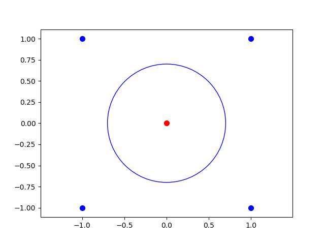
$(-1, 1), \quad (1, 1), \quad (1, -1), \quad (-1, -1)\quad \text{and} \quad (0, 0),$ where $(0, 0)$ is to be separated from the four corners. No line can do it, but a circle

$x^2 + y^2 = r^2, \qquad 0 < r < \sqrt{2}, \tag{9.12}$ certainly can:

Under the map $\varphi(x, y) = (x^2, y^2)$ something drastic happens: all four corners land on the same point $(1, 1)$ , while $(0, 0)$ stays put. Separating two points is no challenge — and pulling a separating line $x_1 + y_1 = r^2$ back through $\varphi$ gives exactly the circle (9.12) . The right map does not just help; it can make the problem trivial.

The general recipe is now clear: find a map

$\varphi: \RR^d\rightarrow \RR^N,$ such that the transformed data

$(\varphi(x_1), y_1), \dots, (\varphi(x_m), y_m)$ becomes linearly separable, and run the machinery of Theorem 9.8 in $\RR^N$ . When the coordinates of $\varphi$ are monomials, the optimal hyperplane $\alpha^\top \varphi(v) + \beta = 0$ upstairs is an intricate polynomial curve downstairs.

The cell below shows the recipe at full power. It scatters random points in the plane, labels them by which side of the snaky cubic curve $y = \frac{x^3 - 2 x}{2}$ they fall on, lifts them to $\RR^9$ using all monomials of degree at most three,

$\varphi(x, y) = (x,\, y,\, x y,\, x^2,\, y^2,\, x^3,\, x^2 y,\, x y^2,\, y^3),$ and hands the lifted points to the support vector machine with kernel="linear" — a plain hyperplane in $\RR^9$ , nothing we have not seen before. Pulled back to the plane, that hyperplane is the black cubic curve in the plot, hugging the gap in the data and separating the two clusters perfectly — carried, as always, by a handful of support vectors.

Live Python

import numpy as np
import matplotlib.pyplot as plt
from sklearn import svm

rng = np.random.default_rng(3)
P = rng.uniform(-2, 2, size=(300, 2))
vals = P[:, 1] - (P[:, 0]**3 - 2*P[:, 0])/2   # side of the cubic curve
keep = np.abs(vals) > 0.3                     # leave a visible gap
P, labels = P[keep], np.sign(vals[keep])

def phi(x, y):            # all monomials of degree <= 3
    return np.column_stack([x, y, x*y, x**2, y**2,
                            x**3, x**2*y, x*y**2, y**3])

model = svm.SVC(kernel="linear", C=1e6)       # a hyperplane in R^9
model.fit(phi(P[:, 0], P[:, 1]), labels)
print("points:", len(P))
print("training errors:",
      (model.predict(phi(P[:, 0], P[:, 1])) != labels).sum())
print("support vectors:", len(model.support_))

g1, g2 = np.meshgrid(np.linspace(-2, 2, 300), np.linspace(-2, 2, 300))
z = model.decision_function(phi(g1.ravel(), g2.ravel())).reshape(g1.shape)
plt.contourf(g1, g2, z, levels=20, cmap="coolwarm", alpha=0.75)
plt.contour(g1, g2, z, levels=[0], colors="black")
plt.scatter(*P[labels == 1].T, color="red", s=22, edgecolor="black")
plt.scatter(*P[labels == -1].T, color="blue", s=22, edgecolor="black")
plt.gca().set_aspect("equal")
plt.show()

There is a catch. For interesting data the dimension $N$ explodes: degree three in two variables already took $9$ coordinates, and higher degrees in more variables quickly outgrow any computer.

The dual optimization problem comes to the rescue. In (9.10) the number of variables is the number of data points $m$ — not $N$ — and the transformed data enter only through the $m\times m$ matrix

$D_{ij} = y_i y_j\, \varphi(x_i)\cdot \varphi(x_j). \tag{9.13}$ The dimension $N$ appears nowhere, provided we find a clever way of getting our hands on the dot products $\varphi(x_i)\cdot \varphi(x_j)$ in (9.13) without ever computing $\varphi$ itself. Here an old concept from pure mathematics called kernel functions helps us.

9.2.5 Kernel functions

A kernel function is a function $k: \RR^d\times \RR^d \rightarrow \RR$ , that is a hidden dot product in the following sense: there exists a function

$\varphi: \RR^d\rightarrow \RR^N,$ such that

$k(u, v) = \varphi(u)\cdot \varphi(v). \tag{9.14}$

Let $k:\RR^2 \times \RR^2 \rightarrow \RR$ be given by

$k(u, v) = (u^\top v + 1)^2.$ Then

$\begin{aligned} k((x_1, y_1), (x_2, y_2)) &= (x_1 x_2 + y_1 y_2 +1)^2\\ &= x_1^2 x_2^2 + y_1^2 y_2^2 + 2 x_1 x_2 y_1 y_2 + 2 x_1 x_2 + 2 y_1 y_2 + 1. \end{aligned}\tag{9.15}$ One gleans from (9.15) that $k$ is a kernel function, since (9.14) is satisfied for $\varphi: \RR^2\rightarrow \RR^6$ given by

$\varphi(a, b) = (a^2, b^2, \sqrt{2} a b, \sqrt{2} a, \sqrt{2} b, 1).$

Once we have a kernel function for $\varphi$ we can replace the matrix in (9.13) by

$D_{ij} = y_i y_j\, k(x_i, x_j)$

and proceed to solve the optimization problem without worrying about the sometimes insurmountable size of $\RR^N$ .

The kernel of Example 9.18 is built into sklearn as kernel="poly", degree=2, coef0=1. The cell below turns it loose on the five points from the beginning of this subsection, where $(0, 0)$ had to be separated from the four corners. The support vector machine — solving the dual optimization problem with the kernel in place of the dot product — finds a closed separating curve, and we never leave $\RR^2$ to compute in $\RR^6$ .

Live Python

Compare the black curve with the circle (9.12) you would draw by hand — and with the curve you will compute in the kernel perceptron exercise below.

9.2.6 The Gaussian kernel and infinite dimension

The most famous kernel of all is the Gaussian kernel

$k(u, v) = e^{-|u - v|^2},$ known to sklearn as kernel="rbf" (for radial basis function). Which map $\varphi$ hides behind this one? Let us look in dimension one, where the answer is both elementary and dizzying. Using the series $e^t = \sum_{k=0}^\infty \frac{t^k}{k!}$ of the exponential function on the last factor in $e^{-(u - v)^2} = e^{-u^2} e^{-v^2} e^{2 u v}$ , we get

$e^{-(u - v)^2} = \sum_{k=0}^\infty \left( \sqrt{\frac{2^k}{k!}}\, e^{-u^2} u^k \right) \left( \sqrt{\frac{2^k}{k!}}\, e^{-v^2} v^k \right).$ This says precisely that $k(u, v) = \varphi(u)\cdot \varphi(v)$ for

$\varphi(u) = e^{-u^2} \left(1,\ \sqrt{2}\, u,\ \sqrt{\tfrac{2^2}{2!}}\, u^2,\ \sqrt{\tfrac{2^3}{3!}}\, u^3,\ \dots \right)$ — one coordinate for every power of $u$ .

The feature space behind the Gaussian kernel is infinite dimensional. No computer could store a single vector $\varphi(u)$ , let alone find a separating hyperplane among such vectors. And none has to: the dual problem only ever asks for the numbers $k(x_i, x_j)$ — one exponential each. The support vector machine quietly optimizes over an infinite dimensional space while your laptop multiplies small matrices. A similar expansion works in $\RR^d$ for every $d$ .

There is also a completely down-to-earth way of viewing the resulting classifier. As in (9.9) , the optimal normal vector is a linear combination of the transformed support vectors, so a new point $v$ is classified by the sign of

$\alpha^\top \varphi(v) + \beta = c_1\, e^{-|v - x_1|^2} + \cdots + c_m\, e^{-|v - x_m|^2} + \beta$ for suitable numbers $c_i$ , non-zero only at the support vectors: a landscape of Gaussian hills (where $c_i > 0$ ) and valleys (where $c_i < 0$ ), with the separating curve at sea level. With enough hills and valleys any coastline can be traced, which is why the Gaussian kernel separates essentially any labeled data set.

The cell below turns it loose on data that would humiliate any polynomial of modest degree: two interlocking spirals. The background coloring is exactly the landscape $\alpha^\top \varphi(v) + \beta$ , and the black curve is sea level.

Live Python

import numpy as np
import matplotlib.pyplot as plt
from sklearn import svm

rng = np.random.default_rng(1)
t = np.linspace(np.pi/4, 3*np.pi, 100)
spiral = np.column_stack([t*np.cos(t), t*np.sin(t)]) / 3
X = np.vstack([spiral + rng.normal(0, 0.06, spiral.shape),
               -spiral + rng.normal(0, 0.06, spiral.shape)])
y = np.array([1]*len(t) + [-1]*len(t))

# gamma tunes the width: k(u, v) = exp(-gamma |u - v|^2)
model = svm.SVC(kernel="rbf", gamma=2.0, C=10.0)
model.fit(X, y)
print("training errors:", (model.predict(X) != y).sum())
print("support vectors:", len(model.support_), "of", len(X))

g1, g2 = np.meshgrid(np.linspace(-3.4, 3.4, 400),
                     np.linspace(-3.4, 3.4, 400))
z = model.decision_function(
        np.column_stack([g1.ravel(), g2.ravel()])).reshape(g1.shape)
plt.contourf(g1, g2, z, levels=24, cmap="coolwarm")
plt.contour(g1, g2, z, levels=[0], colors="black", linewidths=2)
plt.scatter(*X[y == 1].T, color="red", s=16, edgecolor="black")
plt.scatter(*X[y == -1].T, color="blue", s=16, edgecolor="black")
plt.gca().set_aspect("equal")
plt.show()

Zero training errors on the two spirals, and the landscape in the picture is built from one Gaussian hill or valley per support vector — the cell prints how many there are (a substantial share of the $200$ points; wiggly boundaries are expensive). Everything computed in $\RR^2$ , everything happening in $\RR^\infty$ .

9.2.7 The kernel perceptron algorithm

Recall the stunningly simple perceptron algorithm from section 5.3.2 . This algorithm can be modified to handle non-linear separation too by using kernel functions. In fact, this modification was one of the inspirations for the development of the support vector machines described above.

After having mapped a set of vectors $x_1, \dots, x_m\in \RR^d$ with labels $y_1, \dots, y_m\in\{\pm 1\}$ to $\varphi(x_1), \dots, \varphi(x_m)$ , via $\varphi:\RR^d\rightarrow \RR^N$ , we are looking for a vector $w\in \RR^N$ , such that

$\begin{aligned} w^\top \varphi(x_i) &> 0\quad\text{if}\quad y_i = 1\\ w^\top \varphi(x_i) &< 0\quad\text{if}\quad y_i = -1. \end{aligned}\tag{9.16}$ Such a vector is expressible as

$w = \lambda_1 \varphi(x_1) + \cdots + \lambda_m \varphi(x_m).$ The (dual) perceptron algorithm works adjusting the coefficients $\lambda_1, \dots, \lambda_m$ successively as follows: if $w^\top$ is wrong about the placement of $\varphi(x_j)$ in (9.16) i.e., if $y_j w^\top \varphi(x_j) < 0$ , then let

$\lambda_j := \lambda_j + y_j.$ If we have a kernel function $k$ for $\varphi$ , then

$w^\top \varphi(x_j) = w\cdot \varphi(x_j) = \sum_{i=1}^m \lambda_i \varphi(x_i)\cdot \varphi(x_j) = \sum_{i=1}^m \lambda_i k(x_i, x_j)$ and we can use the kernel function in the algorithm without resorting to computing $\varphi$ and the inner product in $\RR^N$ .

Use the kernel function in Example 9.18 and the kernel perceptron algorithm to separate

$((-1, -1), -1), \quad ((-1, 1), -1), \quad ((1, -1), -1), \quad ((0,0), 1), \quad ((1, 1), 1).$ Sketch the points and the separating curve.

9.3 Interior point methods

The support vector machines of the previous section simply called sklearn, which solved the optimization problem of Theorem 9.8 for us in milliseconds. But how? For the record, sklearn attacks the dual problem (9.10) with sequential minimal optimization (SMO): repeatedly pick two of the multipliers $\lambda_i, \lambda_j$ — two at a time, since the constraint $\Lambda^\top Y = 0$ must be preserved — and improve them by solving the resulting two-variable problem, for which there is a closed formula. That the dual has one variable per data point and touches the data only through the matrix $D$ is precisely what makes this fast, kernels included. So the dual problem of Section 9.1 is not just theory; it is what actually runs on your machine.

In this section we develop a different, completely general method for constrained convex optimization — the classical workhorse known as the interior point method. There is a very nice trick (probably going back to von Neumann) for solving constrained optimization problems of the form

$\minunder{(x_1, \dots, x_d)\in C}\; f(x_1, \dots, x_d), \tag{9.17}$ where $C$ is defined by the differentiable functions $g_i:\RR^d\rightarrow \RR$ as

$C = \{v\in \RR^d \mid g_1(v) \leq 0, \dots, g_m(v)\leq 0\}.$ The functions $g_i$ define the boundary (or barrier) of $C$ . We use them to define the logarithmic barrier function

$B(v) = - \sum_{i=1}^m \log(-g_i(v))$ defined on the interior

$C^o = \{v\in \RR^d \mid g_1(v) < 0, \dots, g_m(v) < 0\}.$ The boundary of $C$ is

$\partial C = \{v\in C \mid g_1(v) = 0 \vee \cdots \vee g_m(v) = 0\}.$ You can see that the logarithmic barrier function explodes (becomes unbounded), when a vector $v\in C^o$ approaches $\partial C$ , since $-\log(t)$ is unbounded as $t\to 0$ for $t>0$ .

The cool idea is to consider the function

$f_\epsilon(v) = f(v) + \epsilon B(v) \tag{9.18}$ for $\epsilon > 0$ . This function has a global minimum $v_\epsilon\in C^o$ .

Prove that $f_\epsilon$ is a convex function if $f$ and $g_1, \dots, g_m$ are convex functions.

Hint

Prove and use that if $f$ is a decreasing convex function (in one variable) and $g$ is a convex function, then $f(-g(x))$ is a convex function, where we assume the composition makes sense.

The upshot is that $v_\epsilon \to v_0$ as $\epsilon\to 0$ . This is the content of the following theorem, which we will not prove.

Let $v_\epsilon$ be a point in $C^o$ with

$f_\epsilon(v_\epsilon) = \min\left\{ f_\epsilon(v) \middle| v\in C^o \right\}$ for $\epsilon > 0$ and $f^* = \min\left\{ f(v) \middle| v\in C \right\}$ . Then

$0\leq f(v_\varepsilon) - f^* \leq \varepsilon m$ and $f(v_\varepsilon)\to f^*$ as $\varepsilon \to 0$ . If (9.17) has a unique optimum $v^*$ , then by using $\epsilon=\frac1n$ we obtain a sequence $v_{\frac{1}{n}}\to v^*$ as $n\to \infty$ .

We move on to give concrete examples of Theorem 9.21 in action.

9.3.1 Quadratic function with polyhedral constraints

A much used setup in optimization is minimizing a quadratic functions subject to polyhedral constraints. This is the optimization problem

$\minunder{A v\, \leq\, b}\; v^\top Q v + c^\top v, \tag{9.19}$ where $Q$ is a $d\times d$ matrix, $A$ is an $m\times d$ matrix, $c\in \RR^d$ and $b\in \RR^m$ .

Certainly the constraints $A v\leq b$ define a convex subset of $\RR^d$ , but the function $v^\top Q v + c^\top v$ is not strictly convex unless $Q$ is positive definite. If $Q$ is not positive semidefinite (9.19) is difficult.

If $Q$ is positive semidefinite, the interior point method outlined above usually works well.

The optimization problem (9.2) has the form (9.19) , when we put

$\begin{aligned} Q &= \begin{pmatrix} 1 & 0 & 0\\ 0 & 1 & 0\\ 0 & 0 & 0 \end{pmatrix}\\ c &= \begin{pmatrix} 0 \\ 0 \\ 2 \end{pmatrix}\\ A &= \begin{pmatrix} -2x_1 & -2y_1 & -1\\ \vdots & \vdots & \vdots \\ -2x_n & -2y_n & -1 \end{pmatrix}\\ b &= \begin{pmatrix} -x_1^2 - y_1^2\\ \vdots \\ -x_n^2 - y_n^2 \end{pmatrix} \end{aligned}$

Show that the optimization problem in Theorem 9.8 also has the form (9.19) by writing up the matrices $Q$ and $A$ and the vectors $c$ and $b$ for the labeled points $(v_1, y_1), \dots, (v_m, y_m)$ with $v_i\in \RR^d$ .

Quadratic optimization problems, such as the one in Theorem 9.8 , can be solved numerically in python. The code below uses the function minimize from scipy. It attempts (in general) to solve the optimization problem

$\minunder{G x\, \leq\, h\\[2pt] A x\, =\, b}\; \frac{1}{2} x^\top Q x + p^\top x.$

In the cell below the optimization problem

$\minunder{x_1\, \geq\, 0,\;\; x_2\, \geq\, 0\\[2pt] x_1 + x_2\, =\, 1}\; 2 x_1^2 + x_2^2 + x_1 x_2 + x_1 + x_2$ has been entered.

Live Python

Take a look at the input format in Example 9.24 . Can you tell which optimization problem in this chapter is solved below? Compare the numerical solution with your solution to the exercise below Example 9.9 .

Live Python

Let us watch Theorem 9.21 in action on the fire station problem of Example 9.3 : find the smallest circle enclosing the seven houses

$(0, 0), \quad (2,2), \quad (-3, 2), \quad (1, 0), \quad (-2, 1), \quad (-1, 3) \quad\text{and}\quad (0, 4).$ The cell below minimizes the barrier function $f_\epsilon$ from (9.18) for the constraints of (9.2) with

$\epsilon = 1,\quad 0.1,\quad 0.01,\quad 0.001,\quad 0.0001,$ each unconstrained minimization done by minimize from scipy as in Example 9.24 , and each starting from the minimum $v_\epsilon$ found for the previous $\epsilon$ — a warm start, which is how interior point methods work in practice. Watch the printed output converge to the exact solution: the circle of radius $\frac{5}{2}$ centered at $\left(-\frac{1}{2}, 2\right)$ , touching the three houses $(2,2)$ , $(-3,2)$ and $(1,0)$ . The plot shows the shrinking dashed circles closing in on the optimal solid one, and in red the path $\epsilon \mapsto v_\epsilon$ — the celebrated central path of interior point methods.

Live Python

import numpy as np
import matplotlib.pyplot as plt
from scipy.optimize import minimize

# the houses from Example above
pts = np.array([[0, 0], [2, 2], [-3, 2], [1, 0],
                [-2, 1], [-1, 3], [0, 4]], dtype=float)

def f_eps(v, eps):        # the barrier function for (opt2)
    x, y, lam = v
    g = pts[:, 0]**2 + pts[:, 1]**2 - 2*pts[:, 0]*x - 2*pts[:, 1]*y - lam
    if np.any(g >= 0):
        return np.inf     # infinite outside the interior of C
    return x**2 + y**2 + lam - eps*np.log(-g).sum()

v = np.array([0.0, 0.0, 30.0])     # strictly feasible: a huge circle
path = []
for eps in [1, 0.1, 0.01, 0.001, 0.0001]:
    v = minimize(f_eps, v, args=(eps,), method="Nelder-Mead",
                 options={"xatol": 1e-9, "fatol": 1e-12,
                          "maxiter": 6000}).x
    x, y, lam = v
    r = np.sqrt(lam + x**2 + y**2)   # lam = r^2 - x^2 - y^2
    path.append((x, y, r))
    print(f"eps = {eps:<7}  center = ({x: .4f}, {y: .4f})  "
          f"radius = {r:.4f}")

t = np.linspace(0, 2*np.pi, 200)
for k, (x, y, r) in enumerate(path):
    style = "-" if k == len(path) - 1 else "--"
    plt.plot(x + r*np.cos(t), y + r*np.sin(t), style, color="gray")
plt.plot(*pts.T, "ko")
plt.plot([p[0] for p in path], [p[1] for p in path], "r.-")
plt.gca().set_aspect("equal")
plt.show()

If you are curious about the real algorithmic machinery — Newton's method from the previous chapter with exact line search applied to $f_\epsilon$ — see Section 10.5.1 of my book Undergraduate Convexity.

Solve the two optimization problems in each of the Exercises 7.48 , 7.49 and 7.50 numerically with minimize from scipy as in Example 9.24 (a maximum is found by minimizing $-f$ ). Check the numerical output by actually solving the exercises.

Compute the best line separating the labeled data

((1, 0), +1), ((2, 0), +1), ((3, 0), +1), ((3, 2), +1), ((1, 1), -1), ((2, 2), -1).

using the support vector machine cell from Section 9.2 . Which of the six points are the support vectors?

The interior point method delivers approximations $v_\epsilon$ marching toward the optimum. The rest of the chapter treats the complementary, exact question: given a point $v_0$ , how do we recognize — and certify with a proof — that it is optimal?

9.4 A geometric optimality criterion

Consider the general optimization problem

$\minunder{(x_1, \dots, x_d)\in C}\; f(x_1, \dots, x_d), \tag{9.20}$ where $C$ is a subset of $\RR^d$ .

Suppose that $C\subseteq \RR^d$ is a convex subset and $f:\RR^d\rightarrow \RR$ a differentiable function in (9.20) . If $v_0\in C$ is an optimal solution of (9.20) , then

$\nabla f (v_0) (v - v_0) \geq 0\qquad\text{for every } v\in C. \tag{9.21}$ If $f$ in addition is a convex function, then (9.21) implies that $v_0$ is optimal.

Proof

If $v_0$ is an optimal solution and $v\in C\setminus\{v_0\}$ , then

$\begin{aligned} 0 &\leq f((1-t)v_0 + t v) - f(v_0) = f(v_0 + t(v-v_0)) - f(v_0)\\ &= t\,\left(\nabla f(v_0)(v-v_0) + \epsilon(t (v-v_0)) \abs{v-v_0 }\right) \end{aligned}$ for every $t$ with $0\leq t \leq 1$ , where $\epsilon$ denotes the epsilon function in the definition of differentiability (see Definition 7.3 ). Therefore

$\nabla f(v_0)(v-v_0) + \epsilon(t (v-v_0)) \abs{ v-v_0 }\geq 0$ for $0\leq t\leq 1$ . This is only possible if $\nabla f(v_0)(v-v_0)\geq 0$ . We have silently applied the convexity of $C$ and the differentiability of $f$ at $v_0$ .

If $f$ in addition is convex and (9.21) holds, then Theorem 8.23 shows that $v_0$ is an optimal solution.

A nice application of Proposition 9.28 is where the constraints in $C$ are linear. Then you can test if $v_0$ is an optimal solution by solving the linear program

$\min \nabla f(v_0) v$ for $v\in C$ . If the optimal value is $\geq \nabla f(v_0) v_0$ , then $v_0$ is an optimal solution.

Let us test drive this on the convex optimization problem

$\minunder{x\, \geq\, 0,\;\; y\, \geq\, 0\\[2pt] x + y\, \leq\, 2}\; f(x, y),$ where $f(x, y) = (x-2)^2 + (y-1)^2$ and $\nabla f(x, y) = (2x - 4,\, 2y - 2)$ . The constraints are linear: $C$ is the triangle with vertices $(0,0)$ , $(2, 0)$ and $(0, 2)$ .

Is the vertex $v_0 = (2, 0)$ an optimal solution? Here $\nabla f(v_0) = (0, -2)$ , so the linear program to solve is

$\minunder{(x,\, y)\in C}\; -2y.$ A linear function attains its minimum over the triangle at a vertex (this is the content of the exercise below), so we only have to check three points: $-2y$ takes the values $0$ , $0$ and $-4$ at $(0,0)$ , $(2,0)$ and $(0,2)$ . The optimal value $-4$ is smaller than $\nabla f(v_0)\, v_0 = 0$ , so the test fails — and it fails informatively. For $v = (0, 2)$ we have $\nabla f(v_0)(v - v_0) = -4 < 0$ , so by Proposition 9.28 the vertex $v_0 = (2,0)$ is not optimal: $f$ decreases along the edge from $(2,0)$ toward $(0,2)$ .

Let us instead try $v_0 = \left(\frac{3}{2}, \frac{1}{2}\right)$ , which lies on the same edge. Now $\nabla f(v_0) = (-1, -1)$ and the linear program is

$\minunder{(x,\, y)\in C}\; -x - y$ with the values $0$ , $-2$ and $-2$ at the three vertices: the optimal value is $-2$ . Since

$-2 \geq \nabla f(v_0)\, v_0 = -\tfrac{3}{2} - \tfrac{1}{2} = -2,$ the test succeeds and Proposition 9.28 (here we use that $f$ is convex) certifies that $\left(\frac{3}{2}, \frac{1}{2}\right)$ is an optimal solution — no further theory needed, just one linear program.

The cell below shows both verdicts geometrically. The level sets of $f$ are circles around the unconstrained minimum $(2, 1)$ . The dotted red circle is the level set through $(2, 0)$ : it dips into the triangle, so $C$ contains points with smaller $f$ -value and $(2, 0)$ cannot be optimal — the red arrow is the descent along the edge found by the failed test. The green circle is the level set through $\left(\frac{3}{2}, \frac{1}{2}\right)$ : it only touches the triangle. It is tangent to the edge $x + y = 2$ , and the tangent line is exactly the hyperplane $\nabla f(v_0)\, v = \nabla f(v_0)\, v_0$ from Proposition 9.28 — compare with the picture for a curved boundary in the next example.

Live Python

import numpy as np
import matplotlib.pyplot as plt

f = lambda x, y: (x - 2)**2 + (y - 1)**2

fig, ax = plt.subplots(figsize=(6.5, 6))

# the triangle C
tri = np.array([[0, 0], [2, 0], [0, 2], [0, 0]])
ax.fill(tri[:, 0], tri[:, 1], color="lightsteelblue", alpha=0.6)
ax.plot(tri[:, 0], tri[:, 1], color="steelblue", linewidth=2)

# level circles of f around the unconstrained minimum (2, 1)
x, y = np.meshgrid(np.linspace(-0.7, 3.5, 400), np.linspace(-1.3, 2.7, 400))
ax.contour(x, y, f(x, y), levels=[0.1, 2.0, 3.5],
           colors="gray", linestyles="dashed", linewidths=1)
ax.contour(x, y, f(x, y), levels=[0.5],    # through (3/2, 1/2):
           colors="green", linewidths=2)   # tangent to the edge
ax.contour(x, y, f(x, y), levels=[1.0],    # through (2, 0):
           colors="red", linestyles="dotted", linewidths=1.5)

ax.plot([2], [1], "k*", markersize=13)     # unconstrained minimum
ax.annotate("$(2, 1)$", (2, 1), textcoords="offset points", xytext=(9, 5))
ax.plot([2], [0], "ro", markersize=7)
ax.annotate("$(2, 0)$: not optimal", (2, 0),
            textcoords="offset points", xytext=(9, -14), color="red")
ax.plot([1.5], [0.5], "go", markersize=7)
ax.annotate("$(3/2, 1/2)$: optimal", (1.5, 0.5),
            textcoords="offset points", xytext=(-120, 14), color="green")

# the descent along the edge found by the failed test at (2, 0)
ax.annotate("", xy=(1.62, 0.38), xytext=(2, 0),
            arrowprops=dict(arrowstyle="->", color="red", lw=2))

ax.set_aspect("equal")
ax.set_xlim(-0.7, 3.5)
ax.set_ylim(-1.3, 2.7)
plt.show()

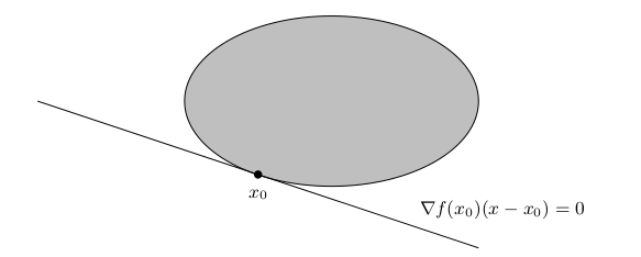
Proposition 9.28 also applies when the boundary of $C$ is curved, as in the optimization problem

$\minunder{x^2 + y^2\, \leq\, \frac{1}{2}}\; (x+1)^2 + (y+1)^2.$

Here Proposition 9.28 shows that $v_0=\left(-\tfrac{1}{2}, -\tfrac{1}{2}\right)$ is optimal: with $\nabla f(v_0) = (1, 1)$ , the hyperplane

$\nabla f(v_0)\, v = \nabla f(v_0)\, v_0,$ which is the line $x + y = -1$ , touches the boundary of

$C = \left\{(x, y)\in \RR^2 \,\middle|\, x^2 + y^2\leq \tfrac{1}{2}\right\}$ exactly at $v_0$ , and $C$ lies on the side where $\nabla f(v_0)(v - v_0) \geq 0$ — as sketched below.

Sketch how Proposition 9.28 applies to show that an optimum in a linear programming problem

$\minunder{A \begin{pmatrix} x \\ y \end{pmatrix} \leq\, b}\; c x + d y$ in the plane $\RR^2$ always can be found in a vertex.

Let $f:\RR^2\rightarrow \RR$ be a differentiable convex function and

$S =\Set{ (x, y) }{ -1 \leq x \leq 2, -1 \leq y \leq 1 }.$ Suppose that $\nabla f(v_0) = (1,0)$ for $v_0 = (-1,\frac{1}{2})$ . Prove that $v_0$ is a minimum for $f$ defined on $S$ .

Guess the solution to the optimization problem

$\min\Set{ (x-5)^2 + (y-5)^2\, }{ \, x\geq 0,\, y\geq 0,\, x^2 + y^2 \leq 25 }.$ Show that your guess was correct!

9.5 The KKT conditions

The KKT in the title of this section is short for Karush-Kuhn-Tucker.

We will limit ourselves to a convex optimization problem of the form

$\minunder{(x_1, \dots, x_d)\in C}\; f(x_1, \dots, x_d), \tag{9.22}$ where $C$ is defined by the differentiable convex functions $g_i:\RR^d\rightarrow \RR$ for $i = 1, \dots, m$ as

$C = \{v\in \RR^d \mid g_1(v) \leq 0, \dots, g_m(v)\leq 0\}$ and $f:\RR^d\rightarrow \RR$ is a convex function.

To the optimization problem (9.22) we associate the (famous) Karush-Kuhn-Tucker (KKT) conditions:

$\begin{aligned} &\lambda_1 \geq 0, \dots, \lambda_m\geq 0\\ \\ &g_1(v_0)\leq 0, \dots, g_m(v_0)\leq 0\\ \\ &\lambda_1 g_1(v_0) = 0, \dots, \lambda_m g_m(v_0) = 0\\ \\ &\nabla f(v_0) + \lambda_1 \nabla g_1(v_0) + \cdots + \lambda_m \nabla g_m(v_0) = 0. \end{aligned}\tag{9.23}$

Notice that the KKT conditions consist of $2m$ inequalities and $m+d$ equations in the $m+d$ unknowns $\lambda_1, \dots, \lambda_m, v_0 = (x_1, \dots, x_d)$ . The KKT conditions form a surprising theoretical foundation for optimization problems of the type in (9.22) . You should take a peek back to the theory of Lagrange multipliers in section 7.10 and compare with (9.23) .

The KKT conditions associated with the convex optimization problem in Example 9.1 are

$\begin{aligned} \lambda_1, \lambda_2, \lambda_3, \lambda_4 & \geq 0\\ -x -y + 2 &\leq 0\\ y - 2&\leq 0\\ x - 3&\leq 0\\ -y + 1 &\leq 0\\ \lambda_1 (- x - y + 2) &=0\\ \lambda_2 (y - 2) &= 0\\ \lambda_3 (x - 3) &= 0\\ \lambda_4 (-y + 1) &= 0\\ 2 x - \lambda_1 + \lambda_3 &= 0\\ 2 y - \lambda_1 + \lambda_2 -\lambda_4 &= 0. \end{aligned}$

Verify that the KKT conditions of the optimization problem in Example 9.1 are the ones given in Example 9.34 .

To state our main theorem we need a definition.

The optimization problem (9.22) is called strictly feasible if there exists $z_0\in \RR^d$ with

$\begin{aligned} g_1(z_0) &< 0\\ &\vdots\\ g_m(z_0) &< 0. \end{aligned}$

Below is the main result in our limited convex setting. We will not go into the proof, which can be found in my book Undergraduate Convexity.

Let $v_0$ be an optimal solution of (9.22) . If (9.22) is strictly feasible, then the KKT conditions are satisfied at $v_0$ for suitable $\lambda_1, \dots, \lambda_m$ .
If the KKT conditions are satisfied at $z\in \RR^d$ for some $\lambda_1, \dots, \lambda_m$ , then $z$ is an optimal solution to (9.22) .

Let us now touch base with a rather simple example. Consider the optimization problem

$\minunder{x\in [1,\, 2]}\; x. \tag{9.24}$

Here $f(x) = x, g_1(x) = -x + 1$ and $g_2(x) = x - 2$ in (9.22) . Therefore the KKT conditions in (9.23) are

$\begin{aligned} \lambda_1 &\geq 0\\ \lambda_2 &\geq 0\\ -x + 1 &\leq 0\\ x - 2 &\leq 0\\ \lambda_1 (- x + 1) &= 0\\ \lambda_2 (x -2 ) &= 0\\ 1 -\lambda_1 + \lambda_2 &= 0. \end{aligned}\tag{9.25}$

Before even thinking about reading on, you should attempt to find a solution $x, \lambda_1, \lambda_2$ to the above KKT conditions (inequalities) and then verify using Theorem 9.37 (ⅱ) that $x$ is optimal. Also, try only using Theorem 9.37 (ⅰ) and (9.25) to show that $x = 2$ is not a solution to (9.24) .

Consider the convex optimization problem (9.22) and the KKT conditions (9.23) . Which of the following statements are true?

If $\lambda_i > 0$ in a solution of the KKT conditions, then the $i$ -th constraint is active i.e., $g_i(v_0) = 0$ .

If $v_0$ is an optimal solution, then the KKT conditions are satisfied at $v_0$ , even when (9.22) is not strictly feasible.

The KKT conditions can be satisfied at only one point $v_0$ .

If the KKT conditions are satisfied at $z$ , then $z$ is an optimal solution — no strict feasibility needed.

Give an example of a convex optimization problem as in (9.22) , which is not strictly feasible and with an optimal solution $v_0$ that does not satisfy the KKT conditions. Such an example shows that strict feasibility is necessary in Theorem 9.37 (ⅰ) .

9.5.1 Strategy

A general strategy for finding solutions to the KKT conditions in (9.23) is zooming in on (the Lagrange multipliers) $\lambda_1, \dots, \lambda_m$ testing each of them for the two cases $\lambda_i = 0$ and $\lambda_i> 0$ .

One important point, which you can read from (9.23) , is that $g_i(v_0) = 0$ if $\lambda_i > 0$ . To further elaborate, if $\lambda_i > 0$ , then an optimal solution must satisfy $g_i(v_0) = 0$ .

So where exactly in (9.23) is the above claim verified?

The condition $\lambda_i = 0$ simplifies the equations

$\nabla f(v_0) + \lambda_1 \nabla g_1(v_0) + \cdots + \lambda_m \nabla g_m(v_0) = 0$ in (9.23) .

In principle to solve the KKT conditions, one has to try out all the $2^m$ possibilities coming from $\lambda_i = 0$ or $\lambda_i > 0$ for $i=1, \dots, m$ .

Why $2^m$ possibilities above?

How do you solve the optimization problem (or decide there is no solution) if $\lambda_1 = \cdots = \lambda_m = 0$ ?

9.5.2 Example

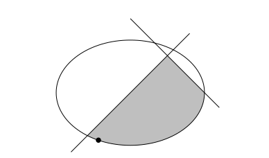
Let $C$ denote the set (see Figure 9.44 ) of points $(x, y)\in \RR^2$ with

$\begin{aligned} x^2 + 2y^2 &\leq 1\\ x + y &\leq 1\\ y &\leq x. \end{aligned}$ We will illustrate the mechanics of solving the KKT conditions in finding an optimal solution for

$\minunder{(x,\, y)\in C}\; x + 3 y. \tag{9.26}$

The convex set $C$ with optimal solution for (9.26) marked.

Putting

$\begin{aligned} g_1(x, y) &= x^2 + 2 y^2 -1\\ g_2(x, y) &= x + y - 1\\ g_3(x, y) &= y - x \end{aligned}$ and $f(x, y) = x + 3y$ , we are in a position to apply Theorem 9.37 , since $g_1, g_2, g_3$ are convex functions and $g_1(z_0) < 0, g_2(z_0)<0, g_3(z_0)<0$ for $z_0 = (0, -\frac{1}{2})$ . This means that an optimal solution of (9.26) satisfies the KKT conditions. The same theorem tells us that the $v_0$ in a solution of the KKT conditions is an optimal solution (here we also use that $f$ is a convex function). The full set of KKT conditions in $x, y, \lambda_1, \lambda_2, \lambda_3\in \RR$ are

$\begin{aligned} x^2 + 2y^2 -1 &\leq 0\\ x + y -1&\leq 0\\ y - x&\leq 0\\ \lambda_1, \lambda_2, \lambda_3 & \geq 0\\ \lambda_1 (x^2 + 2y^2 -1) &=0\\ \lambda_2 (x+y -1) &= 0\\ \lambda_3 (-x + y) &= 0\\ 1 + 2 \lambda_1 x + \lambda_2 - \lambda_3 &= 0\\ 3 + 4\lambda_1 y + \lambda_2 +\lambda_3 &= 0. \end{aligned}$ A strategy for finding a solution to the KKT conditions is trying (the eight) different combinations of strict inequalities in $\lambda_1, \lambda_2, \lambda_3\geq 0$ . You can see from the last two equations that $\lambda_1 = 0$ is impossible. The condition $\lambda_1 > 0$ shows that an optimal solution has to occur on the lower arc in Figure 9.44 . If $\lambda_3 > 0$ , then $x = y$ and $\lambda_2 = 1+3 \lambda_3 > 0$ by the last two equations. This implies $x = y = \frac{1}{2}$ violating $x^2 + 2 y^2 - 1 = 0$ . Therefore $\lambda_3 = 0$ . If $\lambda_2 > 0$ , then $y=1-x$ and $5 + 4 \lambda_1 + 3 \lambda_2 = 0$ by $\lambda_3 = 0$ and the last two equations. Therefore $\lambda_2=0$ . So we are left with the case $\lambda_1 > 0$ and $\lambda_2 = \lambda_3 = 0$ giving

$x = -\frac{1}{2\lambda_1}\qtextq{and} y = -\frac{3}{4 \lambda_1}.$ Inserting this into $x^2 + 2 y^2 - 1 = 0$ we end up with (see Figure 9.44 )

$\lambda_1 = \frac{\sqrt{11}}{2 \sqrt{2}},\quad x = -\sqrt{\frac{2}{11}} \qtextq{and} y = -\frac{3}{\sqrt{22}}.$

Theorem 9.37 is beautiful mathematics. Going through the KKT conditions as above can be quite lengthy if not impossible in practice. As we have seen, there are other methods for (at least) approximating an optimal solution.

9.5.3 Solving the KKT conditions by computer

Lengthy for a human — but look again at the strategy: $2^m$ cases, and each case is nothing but a system of equations together with some sign checks. That is a job for a computer, and sympy can do it with exact arithmetic. The program below is the strategy of this section made executable. For each of the $2^m$ cases it decides, for every constraint, between $\lambda_i = 0$ and $g_i = 0$ (complementary slackness!), solves the resulting equations together with stationarity

$\nabla f(v_0) + \lambda_1 \nabla g_1(v_0) + \cdots + \lambda_m \nabla g_m(v_0) = 0,$ and keeps only solutions passing the remaining KKT inequalities $\lambda_i \geq 0$ and $g_i(v_0)\leq 0$ .

Live Python

from itertools import product
from sympy import symbols, solve, diff

x, y = symbols('x y', real=True)
lam = symbols('lambda1 lambda2 lambda3', real=True)

f = x + 3*y
g = [x**2 + 2*y**2 - 1, x + y - 1, y - x]

# stationarity: grad f + sum lambda_i grad g_i = 0
stationarity = [diff(f, v) + sum(l*diff(gi, v) for l, gi in zip(lam, g))
                for v in (x, y)]

kkt_solutions = []
for active in product([True, False], repeat=len(g)):
    case = [f"g{i+1}=0" if a else f"lambda{i+1}=0"
            for i, a in enumerate(active)]
    eqs = list(stationarity)
    for a, l, gi in zip(active, lam, g):
        eqs.append(gi if a else l)          # complementary slackness
    found = []
    for sol in solve(eqs, [x, y, *lam], dict=True):
        if len(sol) < 5:
            continue                        # underdetermined case
        if all(sol[l] >= 0 for l in lam) and all(gi.subs(sol) <= 0 for gi in g):
            found.append(sol)
    print(", ".join(case), "->", found if found else "no KKT solution")
    kkt_solutions += found

for sol in kkt_solutions:
    print()
    print("optimal solution:", {x: sol[x], y: sol[y]})
    print("optimal value f =", f.subs(sol), "=", float(f.subs(sol)))

Compare with the hand computation above: seven of the eight cases die — for exactly the reasons we found — and the surviving case $\lambda_1 > 0$ , $\lambda_2 = \lambda_3 = 0$ delivers

$x = -\frac{\sqrt{22}}{11} = -\sqrt{\tfrac{2}{11}}, \qquad y = -\frac{3\sqrt{22}}{22} = -\frac{3}{\sqrt{22}}, \qquad \lambda_1 = \frac{\sqrt{22}}{4} = \frac{\sqrt{11}}{2\sqrt{2}},$ the same numbers in a different radical costume, together with the optimal value $f = -\sqrt{22}/2$ . The program is not tied to this example: replace $f$ and the list $g$ (and the symbols) with your own convex optimization problem and it will grind through the cases for you — bearing in mind that the number of cases doubles with every constraint, which is precisely why practical solvers use the barrier and descent methods of the earlier sections instead. You are welcome to check your hand computations in the exercises below against it.

9.5.4 Closing the circle: KKT and the optimal hyperplane

This chapter opened with the optimal separating hyperplane and ends with certificates of optimality — and the two meet. The dual problem (9.10) was presented without derivation, and its two most mysterious ingredients were the linear combination (9.9) and the constraint $\Lambda^\top Y = 0$ . Both fall out of the KKT conditions, and for the two points that Example 9.12 treated with the dual, every step can be done by hand.

Return to the two points of Example 9.9 : $v_1 = (1, 1)^\top$ with label $y_1 = 1$ and $v_2 = (2, 2)^\top$ with label $y_2 = -1$ . This time we keep all three variables $\alpha = (\alpha_1, \alpha_2)^\top$ and $\beta$ of Theorem 9.8 and treat the problem as (9.22) with

$f(\alpha, \beta) = |\alpha|^2 = \alpha_1^2 + \alpha_2^2$ and the two convex constraint functions

$\begin{aligned} g_1(\alpha, \beta) &= 1 - (\alpha^\top v_1 + \beta) \leq 0\\ g_2(\alpha, \beta) &= 1 + (\alpha^\top v_2 + \beta) \leq 0. \end{aligned}$ The problem is strictly feasible — the optimal line scaled up, say $\alpha = (-2, -2)^\top$ and $\beta = 6$ , satisfies both constraints strictly — so by Theorem 9.37 the KKT conditions characterize the optimum exactly.

The gradients with respect to the three variables $(\alpha_1, \alpha_2, \beta)$ are

$\nabla f = (2\alpha_1,\, 2\alpha_2,\, 0), \qquad \nabla g_1 = (-v_1^\top,\, -1), \qquad \nabla g_2 = (v_2^\top,\, 1),$ so the last KKT condition $\nabla f + \lambda_1 \nabla g_1 + \lambda_2 \nabla g_2 = 0$ splits into two parts. The $\alpha$ -part reads

$2\alpha = \lambda_1 v_1 - \lambda_2 v_2 = \lambda_1 y_1 v_1 + \lambda_2 y_2 v_2$ — the mysterious linear combination (9.9) ! That the normal vector is built from the data points, weighted by multipliers and labels, is not an assumption of the dual; it is forced by the KKT conditions. The $\beta$ -part reads

$-\lambda_1 + \lambda_2 = 0, \qquad\text{i.e.}\qquad \lambda_1 y_1 + \lambda_2 y_2 = 0,$ which is exactly the dual constraint $\Lambda^\top Y = 0$ .

Next, complementary slackness. The multipliers cannot vanish: if $\lambda_1 = \lambda_2 = 0$ , the $\alpha$ -part would give $\alpha = 0$ , and then $g_1 \leq 0$ and $g_2 \leq 0$ would demand $\beta \geq 1$ and $\beta \leq -1$ at once. So $\lambda_1 = \lambda_2 > 0$ , and $\lambda_i\, g_i(v_0) = 0$ forces both constraints to hold with equality:

$\alpha^\top v_1 + \beta = 1 \qquad\text{and}\qquad \alpha^\top v_2 + \beta = -1.$ These are the support vector equations. The claim that both dashed lines carry data points — argued after Theorem 9.8 with a paragraph of shifting and rescaling — is here simply complementary slackness.

The rest is arithmetic. Write $\lambda = \lambda_1 = \lambda_2$ . The $\alpha$ -part gives $\alpha = \tfrac{\lambda}{2}(v_1 - v_2) = -\tfrac{\lambda}{2}(1, 1)^\top$ , and subtracting the two support vector equations gives $\alpha^\top (v_1 - v_2) = 2$ , that is $\tfrac{\lambda}{2}\, |v_1 - v_2|^2 = 2$ , so $\lambda = 2$ . Then

$\alpha = \begin{pmatrix} -1 \\ -1 \end{pmatrix} \qquad\text{and}\qquad \beta = 1 - \alpha^\top v_1 = 3,$ and by Theorem 9.37 (ⅱ) the line $x + y = 3$ is certifiably optimal — the same answer as the dual computation in Example 9.12 , now with a certificate attached. (The multiplier $\lambda = 2$ is twice the dual variable $\lambda = 1$ found in Example 9.12 ; the factor is a bookkeeping constant coming from the objective $|\alpha|^2$ versus $\tfrac{1}{2}|\alpha|^2$ , absorbed by (9.9) .)

Every mystery of the dual has now been witnessed at small scale: the linear combination (9.9) is the $\alpha$ -part of KKT stationarity, the constraint $\Lambda^\top Y = 0$ is its $\beta$ -part, and the support vectors are complementary slackness in action. The general derivation of (9.10) — the one we referred to the literature for — is exactly the computation above with $m$ points in place of two.

9.6 Optimization exercises

Below are some exercises especially related to the KKT conditions. In some of the exercises the minimization problem

$\minunder{(x_1, \dots, x_d)\in C}\; f(x_1, \dots, x_d),$ is denoted

$\min\{f(x_1, \dots, x_d) \mid (x_1, \dots, x_d)\in C\}.$ This should cause no confusion.

Consider the optimization problem

$\minunder{x^2 + y^2\, \leq\, 1\\[2pt] (x+1)^2 + (y-1)^2\, \leq\, 1}\; -x + y \tag{9.27}$

Show that (9.27) is a convex optimization problem.
Sketch the set of constraints in $\RR^2$ and show that $\left(-\frac{1}{2}, \frac{1}{2}\right)$ cannot be an optimal solution to (9.27) .
Write up the KKT conditions for (9.27) and explain theoretically (without actually solving them) why they must have a solution.
Now solve (9.27) . Is the solution unique?

Consider the function $f:\RR^3\rightarrow \RR$ given by

$f(x_1, x_2, x_3) = 2 x_1^2 + 3 x_2^2 + 4 x_3^2.$

Show that $f$ is strictly convex.
Let $S \subseteq \RR^3$ denote the subset of points $(x_1, x_2, x_3)\in \RR^3$ satisfying
$\begin{aligned} x_1 + x_2 + x_3 &\geq 1\\ x_1 + 2 x_2 + 3 x_3 &\leq 5 \end{aligned}$ Show that $S$ is a closed convex subset.
Solve the optimization problem
$\minunder{(x_1, x_2, x_3)\in S}\; f(x_1, x_2, x_3) \tag{9.28}$

Let $S\subseteq B \subseteq \RR^3$ , where

$\begin{aligned} S &= \{(x, y, z)\in \RR^3 \mid x^2 + y^2 + z^2 = 1\}\qquad\text{and}\\ B &= \{(x, y, z)\in \RR^3 \mid x^2 + y^2 + z^2 \leq 1\}. \end{aligned}$

Why does the optimization problem

$\minunder{(x,\, y,\, z)\in S}\; x + 2y + z \tag{9.29}$ have a solution?
Find all optimal solutions to (9.29) .
Let $a, b, c\in \RR$ , where at least one of $a, b, c$ is non-zero. Show that an optimal solution to
$\minunder{(x,\, y,\, z)\in B}\; a x + b y + c z$ belongs to $S$ .

Let

$S = \left\{ (x, y)\in \RR^2 \middle| \begin{matrix} -x & - & y & \leq & 0 \\ 2 x & - & y & \leq & 1 \\ -x & + & 2 y & \leq & 1 \end{matrix} \right\}$

Use the KKT conditions to solve the minimization problem
$\min\{ -x - 4 y | (x, y)\in S \}.$
Use the KKT conditions to solve the minimization problem
$\min\{ x + y | (x, y)\in S \}.$

Solve the optimization problem

$\min\left\{x^2 + 2 y^2 + 3 z^2- 2 x z - x y \middle| \begin{matrix} 2x^2 + y^2 + z^2 & \leq & 4 \\ 1 & \geq & x+y+z \end{matrix} \right\}.$

Let $S =\{ (x, y) | 2 x^2 + y^2 \leq 3, \, x^2 + 2y^2 \leq 3 \}$ and $f(x, y) = (x-4)^2 + (y-4)^2$ .

State the KKT conditions for $\min\{ f(x, y) (x, y)\in S \}$ for $(x, y) = (1,1)$ .
Suppose now that $g(x, y) = (x-a)^2 + (y-b)^2$ . For which $a$ and $b$ does $\min\{ g(x, y) | (x, y)\in S \}$ have optimum in $(1,1)$ ? State the KKT conditions when $(a, b) = (1,1)$ .

Let $f:\RR^2\rightarrow \RR$ be given by

$f(x, y) = (x-1)^2+ (y-1)^2 + 2 x y.$

Show that $f$ is a convex function.
Find $\min\{ f(x, y) | (x, y)\in \RR^2 \}$ . Is this minimum unique? Is $f$ a strictly convex function.

Let
$S = \{ (x, y)\in \RR^2 | x + y \leq 0, \quad x - y \leq 0 \}.$
Apply the KKT-conditions to decide if $(-1, -1)$ is an optimal solution to
$\min\{ f(x, y) | (x, y)\in S \}.$
Find
$m = \min\{ f(x, y) | (x, y)\in S \}$ and
$\{ (x, y)\in \RR^2 | f(x, y) = m \}.$

Let $f:\RR^2\rightarrow \RR$ be given by

$f(x, y) = x^2 + y^2 - e^{x-y-1}$ and let

$C =\{ (x, y) | x - y \leq 0 \}.$

Show that $f:\RR^2\rightarrow \RR$ is not a convex function.
Show that $f$ is a convex function on the open subset
$\{ (x, y) \in \RR^2 | x - y< \tfrac{1}{2} \}$ and conclude that $f$ is convex on $C$ .
Show that $v = (0,0)$ is an optimal solution for the optimization problem $\min\{ f(v) | v\in C \}$ . Is $v$ a unique optimal solution here?

Let $f:\RR^4\rightarrow \RR$ be given by

$f(x_1, x_2, x_3, x_4) = (x_1 - x_3)^2 + (x_2 - x_4)^2$ and $C\subseteq \RR^4$ by

$C =\{ (x_1, x_2, x_3, x_4)\in \RR^4 | x_1^2 + (x_2 - 2)^2 \leq 1,\, x_3 -x_4\geq 0 \}.$

Show that $f$ is a convex function. Is $f$ strictly convex?
Show that $C$ is a convex subset of $\RR^4$ .
Does there exist an optimal point $v = (x_1, x_2, x_3, x_4)\in \RR^4$ for the minimization problem
$\minunder{v\in C}\; f(v)$ with $x_3 = x_4 = 0$ ?
Does there exist an optimal point $v = (x_1, x_2, x_3, x_4)\in \RR^4$ for the minimization problem
$\minunder{v\in C}\; f(v)$ with $x_3 = x_4 = 1$ ?

Let

$f(x, y) = (x-1)^2 + y^2$ and

$C =\{ (x, y)\in \RR^2 | -1\leq x \leq 0,\,\, -1 \leq y \leq 1 \}.$ Solve the optimization problem

$\min\{ f(x, y) | (x, y)\in C \}.$

Let $f:\RR^2\rightarrow \RR$ be given by

$f(x, y) = \tfrac{1}{2} x^2+ y^2-2 y+2.$ Below, the minimization problem

$\min\{ f(x, y) | (x, y) \in S \} \tag{9.30}$ is analyzed for various subsets $S\subseteq \RR^2$ .

Show that $f$ is a convex function
Let
$S =\{ (x, y)\in \RR^2 | - x + 2y \leq 1 \}.$ Show that $(-1, 0)\in S$ cannot be an optimal solution to (9.30) . Find an optimal solution to (9.30) .
Find an optimal solution in (9.30) for
$S =\{ (x, y)\in \RR^2 | -x + 2y \geq 1 \}.$
Are the optimal solutions in (2) and (3) unique?

Let $f:\RR^2\rightarrow \RR$ be given by

$f(x, y) = 2x^2 +3 x + y^2 + y.$

Show that $f$ is a convex function and solve the minimization problem $\min\{ f(x, y) | x, y\in \RR \}$ .

Now let
$S = \left\{ (x, y)\in \RR^2 \middle| \begin{matrix} x^2 + (y+1)^2 & \leq & 1 \\ y - x & \leq & 0 \end{matrix} \right\}$ and consider the minimization problem (P) given by
$\min\{ f(x, y) | (x, y)\in S \}.$
Show using the KKT conditions that $(0,0)$ is not optimal for (P).
Find an optimal solution for (P). Is it unique?